Making Quantitative Decisions

Overview

Decision analysis...is the discipline for helping decision makers choose wisely under conditions of uncertainty.

John Schuyler
Risk and Decision Analysis in Projects, 2001

In this chapter we will discuss making project decisions using quantitative methods. We will focus on the so-called decision tree and its companion, the decision table. Quantitative decisions, whether in trees or tables, often employ an interesting extension of statistical methods called Bayes' Theorem. We will take a look at Bayes' Theorem and see how it can help with making decisions conditioned on other decisions and events.

A Project Policy for Decisions

Quantitative decision making is most useful when there is a rational policy for obtaining the outcomes. Rationality, used in this sense, means that the decision is a consequence of all the inputs having been applied systematically to a decision-making methodology. Given the inputs and the methodology, the decision outcomes are predictable. If only it were so easy in real projects!

Decision Policy Elements

Consider what many would say are necessary policy elements in order that quantitative decisions can be made. [1]

Let's start with an obvious one. If we are trying to choose between one project or another, the first element of decision policy is that we would give priority to those projects that are traceable to goals through strategy. If such is the case, we are assured that the deliverables, applied according to the concept of operations, will yield benefits to the business.

Second, all things otherwise being equal, we would decide in favor of that initiative that brings the most financial gain to the business. Now, if the project or initiative is in the public sector, this principle might not be second. Indeed, this principle may not even be a part of the decision policy. But for profit-making businesses, the financial benefit is always available as a tiebreaker.

Third, as among financial benefits, we would decide in favor of those benefits that are measurable consequences of project outcomes. If cause and effect can be established, then we say we have a consequential benefit. Project managers call such benefits "hard benefits." For example, a project targeted as improving operational efficiency has hard benefits if the cost input of the organization is reduced as a result of project activity. However, if the benefit of the project is "avoided increased costs" in the future, then the benefits are said to be "soft." Between two projects with benefits as described above, the former would have precedence over the latter.

Sometimes financial benefits are not specifically estimated. Project managers say that there is no ROI (return on investment) for the project. Such can be the case for projects in the public sector, but so can it also be the case for research projects. Corporate "internal research and development (IR&D)" projects are done many times because we must explore and innovate. The invention of nylon is said to be more of an accident than anything planned. Was going to the moon in the Apollo program decided on the basis of an ROI? No, but there were benefits set for Apollo and its companion Mercury and Gemini programs. As a matter of policy, projects that advance the mission or respond directly to the commitments of senior managers are often selected first.

Policy should dictate that a quantitative statistical estimate of risk be made. Each risk has a downside and an upside. Every manager and every organization has a risk tolerance. Tolerance usually controls the downside. If the downside is unaffordable, the decision may be that the project cannot go forward. So the policy statement is that for projects of equal quantitative risk estimates, the project that is most risk averse is to be selected over projects of greater risk; if the downside risk exceeds a threshold, then the project cannot be selected, even if it is the least risky of all alternatives.

Finally, the policy should always state that projects must be lawful, ethical, and consistent with all regulatory controls and organizational policies. Of course, the latter two are subject to waivers and set-asides by senior authority.

Table 4-1 summarizes the rational decision-making discussion.

Table 4-1: Decision Policy Elements

Policy Element	Policy Justification
Project alternatives traceable to business goals and strategies	Project choices are most supported and more likely to result in recognizable business results when the choices have clear links to the business goals and strategies. Such linkage is all the more important when the project's resources are challenged for reassignment elsewhere, or when project risks call into question the wisdom of proceeding to invest in the project's progress.
Financial advantage is a tie breaker	Almost all projects have some functional benefit to the business. The only common denominator universally recognized and understood by all business managers is the dollar value returned to the business for having done the project. In the face of essentially equal functional benefit to the business, the tie breaker is always the financial advantage brought to the business by the project. The project with greatest advantage is selected.
Hard benefits trump soft benefits	Hard benefits are measurable and tangible and have clear cause-effect relationships to the project; hard benefits are most often measured in dollars and are therefore most easily understood and evaluated by business leaders. Soft benefits have uncertain cause-effect and the benefits to the business are largely functional. Soft benefits are often difficult to reduce to dollars. The "before and after" principle can be invoked to obtain dollars, but the cause-effect ambiguity discounts the dollars calculated in such a method.
Mission trumps financial when directed by senior authority	Sometimes "we have to do it" and the dollars are much less important. Technically speaking, such a decision is not "rational" based on the definition used in this book, but the decision is most certainly rational considered in a larger context often not involving the project manager or sponsor.
The least risky project trumps a more risky project	All else being equal, a project of lesser risk is always chosen over one with more risk.
All alternatives are legal, ethical, and in compliance with regulation and policy	Project choices should reflect the standards of conduct of the organization. American business usually adopts a standard that prohibits behavior that would jeopardize the business and obviate any benefits returned from the project.

A Context for Quantitative Decisions

Figure 4-1 illustrates the space containing policy, method, inputs, and outcomes. Policy we have discussed. Specific methods will be discussed in subsequent sections, but methods are the tools and processes we apply to input to generate outcomes. Processes can invoke or be constrained by policy, such as applying the hurdle rate for internal rate of return (IRR) and being held to the number of years that go into the calculation. Such policies may be project specific or project portfolio specific, with different figures for each. We will discuss IRR and other financial measures in another chapter.

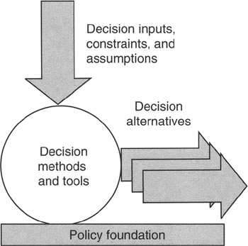
Figure 4-1: Context for Decisions.

Inputs are all the descriptions, data, assumptions, constraints, and experience that can be assembled about a prospective project, event, or alternative that is to be decided. Project managers should have wide latitude to bring any and all relevant material to the decision process. Policy will control the application of input to method, so there is no need to otherwise constrain the assembling of input. The first bit of input needed is a description of the scope of the thing being decided: Is it a choice among projects; a choice among implementation alternatives; a choice of tools, staff, or resources to be applied in a project; or just what? Decisions, by their very nature, are choices among competing alternatives, so a full and complete scope statement of each choice is required. The second component of input is all the attributes of the alternatives. Attributes could include cost, availability, time to develop or deliver, size, weight, color, or any number of other modifiers that distinguish one alternative from another. Third, of course, if there are any constraints (whether physical, logical, mathematical, regulatory, or other), then whatever constraints apply should be scoped and given a full measure of attributes as well.

Once all the inputs, assumptions, experience, and constraints are assembled and organized into separable choices, then a decision methodology can be applied. The fact is that many project managers have trouble organizing the choices and fail to resolve the "if, and, or but" problems of presenting alternatives. However, assembling the choices is the place to stop if the team cannot decide what the alternatives are. If the choices are ambiguous, there is no point in expending the energy to make a decision.

The Utility Concept in Decision Making

When the project manager begins to apply the decision policy to the project situation, the risk attitudes of the decision makers need to be taken into account. If the decision maker is risk neutral, then the decisions will be based on the risk-adjusted estimates without regard to the affordability of the downside or the strategy to exploit the opportunities of the upside. However, decisions are rarely risk neutral if the amount at stake is material to the well being of the organization. In situations where the decision making takes into account the absolute affordability of an opportunity, we call decision making of this type "risk averse." A quantitative view of this concept is embodied in the idea of "utility." Utility simply means that the decision maker's view of risk is either discounted or amplified compared to the risk-neutral view. Figure 4-2 shows this concept. The principal application to projects is evaluating the downside risks attendant to one or more alternatives that are up for a decision. Regardless of the advantageous expected value of a particular opportunity, if its downside is a "bet the company" risk, then the decision may well go against the opportunity.

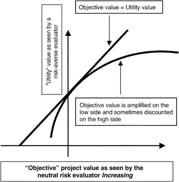
Figure 4-2: Utility Function.

[1]These principles of decision policies are a summarization of the author's experience in many project situations over many years. The material is an expansion of that given in the author's book, Managing Projects for Value. [2]

[1]Goodpasture, John C., Managing Projects for Value, Management Concepts, Vienna, VA, 2001, chap. 3, p. 39.

The Decision Tree

The decision tree is a tool to be applied in a decision methodology. In effect, the decision tree, and its cousin the decision table, sums up all the expected values of each of the alternatives being decided and presents those expected values to the decision maker. At the root of the tree is the decision itself. Extending out from the root is the branch structure representing various paths from the root (decision) to the choices. For those familiar with the "fishbone" diagram from the Total Quality Management toolkit, the decision tree will look very familiar. Along the pathways or branches of the decision tree are quantitative values that are summed along the way at summing nodes. Normally, the project manager makes the decision by following the organization's decision policy in favor of the most advantageous quantitative value. In some cases, deciding most advantageously means picking the larger value, but sometimes the most advantageous value is the smaller one.

The Basic Tree for Projects

Figure 4-3 shows the basic layout. It is customary, as described by John Schuyler in his book, Risk and Decision Analysis in Projects, Second Edition, [3] to show the tree laying on its side with the root to the left. Such an orientation facilitates adding to the tree by adding paper to the right. We use a somewhat standard notation: the square is the decision node; the decision node is labeled with the statement of the decision needed. Circles are summing nodes for quantitative values of alternatives or of different probabilistic outcomes. Diamonds are the starting point for random variables, and the triangle is the starting point for deterministic variables.

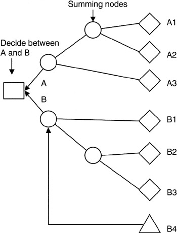
Figure 4-3: Decision Tree.

In Figure 4-3, the decision maker is trying to decide between alternative "A" and alternative "B". There are several components to each decision as illustrated on the far right of the figure. Summing nodes combine the disparate inputs until there is a value for "A" and a value for "B". An example of a decision of this character is well known to project managers: "make or buy a particular deliverable."

Since our objective is to arrive at the decision node with a quantitative value for "A" and "B" so that the project manager can pick according to best advantage to the project, we apply values in the following way:

• Fixed deterministic values, whether positive or negative, are usually shown on the connectors between summing nodes or as inputs to a summing node. We will show them as inputs to the summing node.
• Random variable values are assigned a value and a probability, one such value-probability pair on each connector into the summing node. The summing node then sums the expected value (value * probability) for all its inputs. Naturally, the probabilities of all random variables leading to a summing node must sum to 1. Thus, the project manager must be cognizant of the 1-p space as the inputs are arrayed on the decision tree.

Figure 4-4 shows a simple example of how the summing node works. Alternative "A" is a risky proposition: it has an upside of $5,000 with 0.8 probability, but it has a downside potential of -$3,000 with a 0.2 probability. "A" also requires a fixed procurement of $2,000 in order to complete the scope of "A". The expected value of the risky components of "A" is $3,400. Combined with the $2,000 fixed expenditure, "A" has an expected value of $5,400 at this node. The most pessimistic outcome of "A" at this node is -$1,000: $2,000 - $3,000; the most optimistic figure is $7,000: $2,000 + $5,000. These figures provide the range of threat and opportunity that make up the risk characteristics of "A".

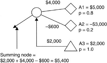
Figure 4-4: Summing Node Detail.

Now, let's add in the possibility of event "A4". The situation is shown in Figure 4-5. If the project team estimates the probability of occurrence of "A4" as 0.4, then the probability of the events on the other leg coming into the final summing node becomes equal to the "1-p" of "A4", or 0.6. Adding risk-weighted values, we come to a final conclusion that the expected value of "A" is $4,840.

Figure 4-5: Summing Node A.

The most pessimistic outcome of "A" at this node remains -$1,000 since if "A2" should occur, "A1" and "A4" will not; the most optimistic figure remains $7,000 since if "A1" occurs, then the other two will not. If "A4" should occur, then "A1" and "A2" will not. However, "A3" is deterministic; "A3" always occurs. So the optimistic value with "A4" is $6,000: $2,000 + $4,000. Obviously, $6,000 is less than the outcome with "A1".

If the analysis of "B" done in similar manner to that of "A" should result in "B" having a value less than $4,840, the decision would be to pick "A". Of course, the risk tolerance of the business must be accommodated. At the decision node there will be an expected value for "A" and another of "B". The project manager can follow the tree branches and determine the most pessimistic outcomes. If the most pessimistic outcomes fit within the risk tolerance of the business, then the outcome, "A" or "B", is decided on the basis of best advantage to the project and to the business. If the most pessimistic outcomes are not within the risk tolerance of the business, and if there is not a satisfactory plan for mitigating the risks to a tolerable level, then the choice of project defaults to the decision policy element of picking on the basis of the risk to the business. Risk managing the most pessimistic outcome is a subject unto itself and beyond the scope of this book.

By now you may have picked up on a couple of key points about decision trees. First, all the Ais and Bis must be identified in order to have a fair and complete input set to the methodology. The responsibility for assembling estimates for the Ais and Bis rests with the project manager and the project team. Second, there is a need to estimate the probability of an occurrence for each discrete input. Again, the project team is left with the task of coming up with these probabilities. The estimating task may not be straightforward. Delphi techniques [4] applied to bottom-up estimates or other estimating approaches may be required. Last, the judgment regarding risk tolerance is subjective. The concept of tolerance itself is subjective, and then the ability of the project team to adequately mitigate the risk is a judgment as well.

A Project Example with Decision Tree

Let's see how a specific project example might work with the decision tree methodology learned so far. Here is the scenario:

• You are the project manager making a make or buy decision on a particular item on the work breakdown structure (WBS). Alternative "A" is "make the item" and alternative "B" is "buy the item."
• There are risks in both alternatives. The primary risk is that if the outcome of either "A" or "B" is late, the delay will cost the project $10,000 per day.
• If you decide to make the item, alternative "A", then there is a fixed materials and labor charge of $125,000. If you decide to buy the item, alternative "B", there is a fixed purchase cost of $200,000. Putting risks aside, "A" seems to be the more attractive by a wide margin.
• Although manufacturing costs are fixed, your team estimates there is a 60% chance the "make" activity will be 20 days late. Your judgment is that you simply do not have a lot of control over in-house resources that do not report to you. However, your team's estimate is that there is only a 20% chance the "buy" activity will be late 20 days, and the purchase price is fixed.

What is your decision? Figure 4-6 shows the decision tree for this project scenario. The decision node is the decision you are seeking: "make or buy." The tree branches lead back through each of the two alternatives. Inputs to the decision-making process are both quantitative and qualitative or judgmental. You know the manufacturing cost, the alternative procurement cost, and the cost of a day's delay in the project. You make judgments about the performance expectations of your in-house manufacturing department and about the performance of an alternative vendor. Perhaps there is a project history you can access of former "similar-to" projects that provide the data for the judgments.

Figure 4-6: Project Decision Example.

As the mathematics show, there is only a $5,000 difference between these two alternatives when all the risk adjustments are factored into the calculation. In fact, the decision favors a "buy" based on the decision policy element to take the alternative of most advantage to the project, just the opposite from the initial conclusion made before risk was taken into account.

How about the downside considerations? If you make the item and the 20-day delay materializes, you are out $325,000. If you buy the item and the 20-day delay happens, you are out $400,000. Since you budget for expected value, either $245,000 or $240,000, the most pessimistic figures provide the information about how much unbudgeted downside risk you are managing:

• Downside risk (buy) ≤ $240,000 - ($200,000 + $200,000) = -$160,000

or

• Downside risk (make) ≤ $245,000 - ($125,000 + $200,000) = -$80,000

You, or your project sponsor, must also decide if the unbudgeted risk is affordable if all risk mitigations fail and the 20-day delay occurs.

Probability Functions in Decision Trees

You might be asking: What about delays other than 20 days, or why 20 days? The project manager and project team may be able to estimate much finer segments than 20 days. There really is no limit to how many individual discrete estimates could be made and summed at a node. It is required that the sum of all probabilities equal 1. So as more discrete estimates are made, say for 1, 2, 5, 10, or other days of delay, the individual probabilities must be made individually less so that the total summation of the "p"s equaling 1 is honored.

Now you may recognize this discussion as similar to the discussion in the chapter on statistics regarding the morphing of the discrete probability distribution into the continuous probability function. Obviously, the values at the input of the summing node are the values from the discrete probability function of the random variable or event that feeds into the summing node. There is no reason that the random variable could not be continuous rather than discrete. There is no reason that the discrete probability function cannot be replaced with a single continuous probability function for the event.

Suppose the inputs to the summing nodes are replaced with continuous probability functions for a continuous random variable. Figure 4-7 shows such a case. Now comes the task of summing these continuous functions. We know we can sum the expected values, and if they are independent random variables, we know we can sum the variances with simple arithmetic. However, to sum the distribution functions to arrive at a distribution function at the decision square is another matter. The mathematics for such a summing task is complex. The best approach is to use a Monte Carlo simulation in the decision tree. For such a simulation you will need software tools, but they are available.

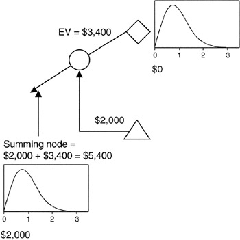
Figure 4-7: Decision Tree with Continuous Distribution.

[3]Schuyler, John, Risk and Decision Analysis in Projects, Second Edition, Project Management Institute, Newtown Square, PA, 2001, chap. 5, p. 59.

[4]The Delphi technique refers to an approach to bottom-up estimating whereby independent teams evaluate the same data, each team comes to an estimate, and then the project manager synthesizes a final estimate from the inputs of all teams.

Decision Tables

Let's see how the example just discussed would look in a decision table. Tables are alternatives to diagrams and often work better than diagrams because they are much easier to work with if the number of summing nodes is more than a couple. Table 4-2 shows the decision we have just worked on in tabular format. Tables, like their diagram counterpart, handle discrete inputs very well, and because tables can easily be computed on spreadsheets or from databases, tables are excellent tools for decision analysis. Maintenance of information is much easier on a spreadsheet or in a database compared to a graphical depiction. We are all familiar with the calculation power of spreadsheets: a single number entry can be recalculated automatically throughout the entire spreadsheet. It is harder to do that with a graphic, which requires less common tools than spreadsheets if a graphic of even small complexity is to be maintained.

Table 4-2: Project Decision Example

Alternative ID	Description	Probability of Schedule Delay	Face Value of Delay, D, @ $10,000 per Day	Expected Value of Delay	Acquisition Cost	Expected Value of Alternative
A	MAKE	0.6 Yes 0.4 No	$200,000 Yes $0 No	$120,000	$125,000	$245,000
B	BUY	0.2 Yes 0.8 No	$200,000 Yes $0 No	$40,000	$200,000	$240,000

For the remaining examples in this book, we will rely more on decision tables. We will use decision trees only when the tree form more easily conveys the concepts we are discussing.

Decisions with Conditions

It would be nice if, but it is rare that, project managers can make decisions without consideration for other activities or constraints going on in the project. Other activities that bear on the decision complicate matters somewhat on the decision tree. Such activities "condition" the decision. Generally, conditions are of two types: independent conditions that establish prerequisites but do not in and of themselves affect performance thereafter, and dependent conditions that do affect performance. An example of an independent condition is that of a sponsor deciding whether or not to exercise a scope option, and then a make-buy decision by the project team that is conditioned only on the sponsor's decision to buy or not.

On the other hand, dependent conditions affect performance or value. That is to say, the performance in a project work package is conditioned on the first decision made. Using the foregoing example, if the sponsor's decision in some way affected the expected value of the maker or provider decision, then the project decision is dependent on the sponsor's decision.

Decisions with Independent Conditions

Let us first discuss the project situation of a decision to be made conditioned on the prior or prerequisite activity of some other work package or some other external event. However, let us say that the alternatives we are deciding between per se are not affected by the prerequisite; just our ability to make decisions about the alternatives is affected.

For illustrating decision making in the context of independent conditions, we will continue with the decision scenario we have been developing in this chapter. The matter before the project team for decision is whether or not to make or buy an item on the WBS. Now, let us impose a condition that is independent of the performance of the in-house manufacturing or of the performance of the vendor if selected:

• The make or buy decision is conditioned on whether or not the project sponsor exercises an option to have the item included in the project deliverables. That is to say, the WBS item in question is optional with the sponsor. It is up to the sponsor to say whether or not it is to be delivered.
• The sponsor's decision is a random variable, S, with values 1 or 0. S = 1 means the item will be included in the project deliverables; S = 0 means it will not be included. Once this prerequisite is satisfied, then the project team can make the decision about make or buy.
• The performance, D, of the subsequent make or buy is independent of the sponsor's decision unless the sponsor decides not to exercise the option for the item. In that case, there would be no subsequent make or buy.
• Our account manager dealing with the sponsor estimates that there is a 75% chance the sponsor will decide in favor of exercising the option for the item. Probability of S = 1 is 0.75. In the "1-p" space there is a 25% chance the sponsor will not exercise the option for the item: probability of S = 0 is 0.25.

Under these new circumstances, what is the decision of the project team, what is the expected value of the item, and what are the downside considerations? We proceed as follows: We must add columns to the decision table to take into account the preconditioning of the sponsor's decision, S, about adding the item to the project deliverables. We then recalculate the outcomes taking special care to account for all events in the "1-p" spaces. Table 4-3 illustrates the results.

Table 4-3: Decision with Independent Conditions

Alternative ID	Description	Probability Sponsor Exercises Option	Sponsor's Decision Value, S	Probability of 20-Day Schedule Overrun	Face Value of Delay, D, @ $10,000 per Day	EV of Delay, D (p of Option * p of Overrun * $Face Value * Sponsor's Decision Value)	EV of Acquisition Cost (p of Option * $Face Value * D)	Expected Value of Alternative
A	MAKE	0.75 Yes 0.75 Yes	1 1	0.6 Yes 0.4 No	$200,000 Yes $0 No	$90,000 = 0.75 * 0.6 * $200,000	$93,750	$183,750
A	MAKE	0.25 No 0.25 No	0 0	0.6 Yes 0.4 No	$200,000 Yes $0 No	$0	$0	$0
B	BUY	0.75 Yes 0.75 Yes	1 1	0.2 Yes 0.8 No	$200,000 Yes $0 No	$30,000 = 0.75 * 0.2 * $200,000	$150,000	$180,000
B	BUY	0.25 No 0.25 No	0 0	0.2 Yes 0.8 No	$200,000 Yes $0 No	$0	$0	$0

Following the mathematics through the table row by row, you can see that the probability of the decision by the sponsor weights the probability of a subsequent delay and weights the acquisition cost. By this we mean that there could only be performance if the sponsor decides favorably to go forward and include the item in the project deliverables. Overall, the probability of delay is the probability that the sponsor makes the decision favorably times the probability of delay given that the decision is favorable. Certainly if the sponsor decides unfavorably, S = 0, so that there is to be no item in the project deliverables, and there is no chance for a delay.

Summing the buy and the make from Table 4-3:

Expected value (buy)	= $0 + $180,000 = $180,000
Expected value (make)	= $0 + $183,750 = $183,750

Under the conditions of the scenario in Tables 4-2 and 4-3, we see that the decision is not changed: it is still "buy." We further see that the expected value of the final decision, $180,000, has a higher unbudgeted downside risk compared to the decision tree without conditions:

Downside risk (make) ≤ $183,750 - ($125,000 acquisition + $200,000 delay) ≤ -$141,250

• Upside (make) = $125,000, the acquisition cost without delay

Downside risk (buy) ≤ $180,000 - ($200,000 acquisition + $200,000 delay) ≤ -$220,000

• Upside (buy) = $200,000, the acquisition cost without delay

The decision tree or table provides the project manager with the expected value of the decision-making process. As we know from previous discussion, expected value is the best single-number representation of a range of uncertainty. Any single instance of the project could fall anywhere in the range. Understanding the range is the purpose of the upside and downside analysis.

Furthermore, the acquisition cost of either alternative ($125,000 for "make" or $200,000 for "buy") has been transformed from deterministic to random by the dependency acquired from the effect of the sponsor's decision. In other words, the sponsor's decision to acquire the item is the random variable, S, with discrete density function S0 = 0, p = 0.25 and S1 = 1, p = 0.75 becomes the density of the acquisition cost, AC:

AC0	=	0, p = 0.25, do not acquire the item
AC1	=	1 * make or buy cost, p = 0.75, acquire the item

Therefore, for decision-making purposes the decision maker would look first to the expected values, weighing first the most advantageous expected value. Then the decision maker would look to the risks and opportunities, downside and upside, and weigh those values in terms of possible effects on the business. The decision policy elements for both risk consideration and expected value are considered jointly in the decision process.

Figure 4-8 shows the "make" part of the scenario we have been discussing. It is evident that decision tree charts grow unwieldy in the face of conditions. Thus, the project team should understand and use tables to simplify matters, especially since tables lend themselves to setup, computation, and maintenance in spreadsheets.

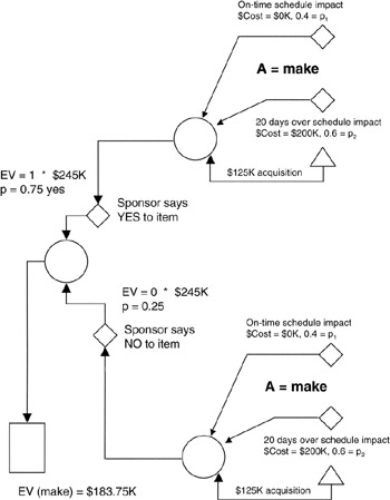
Figure 4-8: Decision Tree with Independent Conditions.

Bayes Theorem

Another degree of complication is introduced when the conditions of performance leading to a decision are interdependent. In this scenario, the probability structure becomes more difficult to manage without a good understanding of dependent probabilities. Thus, we introduce "Bayes' Theorem," named after the English mathematician Thomas Bayes who published his theory, Essay Towards Solving a Problem in the Doctrine of Chances, in 1764. Although Bayes' Theorem can be presented in a couple of forms, it is conveniently shown as follows for project management purposes:

p(A | B) = p(A and B)/p(B)

in which p(A | B) is read as "probability of A given B." Rearranging terms, Bayes' Theorem is also in the following two forms: p(A and B) = p(A | B) * p(B) and p(B) = p(A and B)/p(A | B).

If A and B are independent, then:

p(A | B) = p(A) * p(B)/p(B) = p(A)

because

p(A and B) = p(A) * p(B)

Let's try Bayes' Theorem in natural language with the project examples we have studied so far:

• "The probability of a 20-day delay, D, given a "make" decision, M = 1, is 0.6." In equation form: p(D | M1) = 0.6. If we were interested in solving for p(M1), we would have to estimate p(D and M1).
• "The probability of a 20-day delay, D, given a sponsor's decision, S, to include the item in the project deliverables" is p(D) since D and S are independent.
• "The probability of a 'make' decision, M, given a sponsor's decision, S = 1, to include the item in the project deliverables" is 1.33 * p(M1 and S1). We have no other information about p(M1 | S1) unless we independently measure or estimate p(M1 and S1).

Decision Trees with Dependent Conditions

With Bayes' Theorem in hand, we can proceed to project decisions that are interdependent. Let's continue with our project for which there is an item on the WBS that may or may not be included by the sponsor's decision in the final project scope and for which there is a make or buy decision for satisfying the acquisition to be made by the project team. However, let's change the situation and recognize that a late decision by the sponsor affects the subsequent performance of either make or buy:

• Let SD be the random variable that represents a sponsor's decision that may or may not be delayed beyond a point that the delay affects subsequent make or buy performance or value. In this example, we will say that our confidence in an on-time sponsor's decision is 70%, 0.7. In that event, using our "1-p" analysis, we have p(SD late) = 0.3, 30%.
• If SD is on time, then the situation reverts to a case of independent conditions.

The problem at hand is to determine what is p(Make or Buy performance given SD late). In other words, we need to solve for:

• p(Make performance given SD late) = p(Make performance and SD late/p(SD late)

and

• p(Buy performance given SD late) = p(Buy performance and SD late)/p(SD late)

where performance can be on time or late.

Table 4-4 arrays the scenarios that fall out of the situation in this project. Looking at this table carefully, you will see that there are actually six probabilities since "late or on time" is a shorthand notation for two distinctly different probabilities.

Table 4-4: Dependent Scenarios

Project Situation: MAKE

MAKE 1:

p[MAKE late (or on time) given SD late] = p[MAKE late (or on time) AND SD late]/p(SD late)

MAKE 2:

p[MAKE late (or on time) given SD on time] = p[MAKE late (or on time)]

Project Situation: BUY

BUY 1:

p[BUY late (or on time) given SD late] = p[BUY late (or on time) AND SD late]/p(SD late)

BUY 2:

p[BUY late (or on time) given SD on time] = p[BUY late (or on time)]

Now we come to a vexing problem: to make progress we must estimate the joint probabilities of "make late (or on time) and late SD" and "buy late (or on time) and late SD." We have already said that we have pretty high confidence that SD will be on time, so looking at a joint probability involving "SD late" will be a pretty small space. We do know one thing that is very useful: all the joint probabilities involving "SD late" have to fit in the space of 30% confidence that SD will be late:

• p(Make late and SD late) + p(Make on time and SD late) = p(SD late) = 0.3, or
• p(Buy late and SD late) + p(Buy on time and SD late) = p(SD late) = 0.3

We now must do some estimating based on reasoning about the project situation as we know it. "Make on time" and "Make late" have probabilities of 0.4 and 0.6, respectively. If these were independent of "SD late," then the joint probabilities would multiply out to the multiples of the probabilities:

Make on time and SD late = 0.4 * 0.3 = 0.12

and

Make late and SD late = 0.6 * 0.3 = 0.18

However, in our situation "SD late" conditions performance, so the probabilities are not independent. Intuitively, the joint probability of being on time should be more pessimistic (smaller) since the likelihood of the joint event is more pessimistic than each event acting independently. In that case, the joint probability of being late is more optimistic (more likely to happen):

p(Make on time and SD late) ≤ p(Make on time) * p(SD late),

Estimate: p(Make on time and SD late) = 0.1

and then:

Estimate: p(Make late and SD late) = 0.2 = 0.3 - 0.1

We can make similar estimates for the "buy" situation. Multiplying probabilities as though they were independent gives:

p(Buy late and SD late) = 0.2 * 0.3 = 0.06

and

p(Buy on time and SD late) = 0.8 * 0.3 = 0.24

Following the same reasoning about pessimism as we did in the "make" case:

p(Buy on time and SD late) ≤ p(Buy on time) * p(SD late),

Estimate: p(Buy on time and SD late) = 0.23

and then:

Estimate: p(Buy late and SD late) = 0.07 = 0.3 - 0.23

We now apply Bayes' Theorem to our project situation and calculate the question we started to resolve. The probability p(Make or Buy performance given SD late) is given in Table 4-5 and Table 4-6:

p(Make performance given SD late)	=	p(Make performance and SD late)/p(SD late)
p(Make 20 days late given SD late)	=	0.2/0.3 = 0.67
p(Make 0 days late given SD late)	=	0.1/0.3 = 0.33, and
p(Buy performance given SD late)	=	p(Buy performance and SD late)/p(SD late),
p(Buy 20 days late given SD late)	=	0.07/0.3 = 0.23
p(Buy 0 days late given SD late)	=	0.23/0.3 = 0.77

Table 4-5: Buy Calculations with Dependent Conditions

Project Situation: BUY	Probability of Situation Occurring
20 days and late SD decision	0.07
0 days and late SD decision	0.23
Total LATE SD decision	0.3
20 days and on-time SD decision [*]	0.14
0 days and on-time SD decision[*]	0.56
Total ON-TIME SD decision	0.7
Total SD decision	1.0
20 days given SD late = (20 days and SD late)/SD late	0.23
0 days given SD late = (0 days and SD late)/SD late	0.77
Total given SD late	1.0
20 days given SD on time = 20 days	0.2
0 days given SD on time = 0 days	0.8
Total given SD on time	1.0
[*]These events are independent so the joint probabilities are the product of the probabilities.

Table 4-6: Make Calculations with Dependent Conditions

Project Situation: MAKE	Probability of Situation Occurring
20 days and late SD decision	0.2
0 days and late SD decision	0.1
Total LATE SD decision	0.3
20 days and on-time SD decision [*]	0.42
0 days and on-time SD decision[*]	0.28
Total ON-TIME SD decision	0.7
Total SD decision	1.0
20 days given SD late = (20 days and SD late)/SD late	0.67
0 days given SD late = (0 days and SD late)/SD late	0.33
Total given SD late	1.0
20 days given SD on time = 20 days	0.6
0 days given SD on time = 0 days	0.4
Total given SD on time	1.0
[*]These events are independent so the joint probabilities are the product of the probabilities.

Notice the impact on the potential for being late with a buy. The probability of a 20-day delay has increased from 0.2 with no dependent conditions to 0.23 with dependent conditions. Correspondingly, the on-time prediction dropped from 0.8 to 0.77. For a make decision, the probability of delay went from 0.6 to 0.67.

Let us now compute the dollar value of the outcomes of the decision tables. Table 4-7 provides the illustration of this project scenario. Take care when looking at this table. The acquisition costs of the make, $125,000, or of the buy, $200,000, are not affected by the late or on-time decision, SD, of the sponsor. Acquisition costs are only affected by the sponsor's decision, S, to have the item in the WBS or not. The value of the delay, if any, is taken care of with the value of the timeliness of the decision, SD, times the probability of the decision itself, S.

Table 4-7: Decision with Dependent Conditions

Alternative ID	Description	Probability Sponsor Exercises Option	Probability of Sponsor Decision, SD, Late	Probability of 20-Day Schedule Delay	Face Value of Delay, D, @ $10,000 per Day	EV of Delay, D (p of SD * p of Delay * $Face Value)	EV of Acquisition Cost (p of Option * $Face Value * D)	Expected Value of Alternative
A	MAKE		0.3 Late 0.3 Late	0.67 Yes 0.33 No	$200,000 Yes $0 No	$40,200 $0		= 0.75 * ($40,200
		0.75 Yes					= $125,000 * 0.75	+ $84,000) + $93,750
A	MAKE		0.7 On time 0.7 On time	0.6 Yes 0.3 No	$200,000 Yes $0 No	$84,000 $0	= $93,750	= $186,900
A	MAKE	0.25 No 0.25 No		0.6 Yes 0.4 No	$200,000 Yes $0 No	$0	$0	$0
B	BUY		0.3 Late 0.3 Late	0.23 Yes 0.77 No	$200,000 Yes $0 No	$13,800 $0		= 0.75 * ($13,800
		0.75 Yes					= $200,000 * 0.75	+ $28,000) + $150,000
B	BUY		0.7 On time 0.7 On time	0.2 Yes 0.8 No	$200,000 Yes $0 No	$28,000 $0	= $150,000	= $181,350
B	BUY	0.25 No 0.25 No		0.2 Yes 0.8 No	$200,000 Yes $0 No	$0	$0	$0

Note further that the decision to make or buy is not changed by the effect of a late decision of the sponsor. "Buy" comes out more advantageous in the face of a dependent condition with the sponsor's decision. The upside and downside of a decision in favor of "Buy" are:

Upside of an on-time sponsor's decision is the "Buy" acquisition cost = $200,000

Downside of late sponsor's decision = $181,350 - ($200,000 + $200,000) = -$218,650

Summary of Important Points

Table 4-8 provides the highlights of this chapter.

Table 4-8: Summary of Important Points

Point of Discussion	Summary of Ideas Presented
Project policy for decisions	Quantitative decision making is most useful when there is a rational policy for obtaining the outcomes. Rationality, used in this sense, means that the decision is a consequence of all the inputs having been applied systematically to a decision-making methodology.
Decision trees	The decision tree is a decision tool to be applied in a decision methodology. The decision tree, and its cousin the decision table, sums up all the expected values of each of the alternatives being decided and makes available the expected values to the decision maker. In applying the decision tree to decision making, the project manager gives consideration to risk by considering both the upside opportunity and the downside risk as well as the expected values of the alternatives.
Decisions with independent conditions	It is rare that project managers can make decisions without consideration for other activities or constraints going on in the project. Independent conditions establish prerequisites but do not in and of themselves affect performance thereafter.
Decisions with dependent conditions	Dependent conditions affect performance or value. That is to say, the performance in a project work package is conditioned on the first decision made.
Bayes' Theorem	p(A | B) = p(A and B)/p(B). The project manager usually is given or can estimate directly one of the three probabilities in Bayes' Theorem. To obtain the other two probabilities, usually another estimate or measurement must be made.
Utility	In situations where the decision making takes into account the absolute affordability of an opportunity, we call decision making of this type "risk averse." Utility simply means that the decision maker's view of risk is either discounted or amplified compared to the risk-neutral view.

References

1. Schuyler, John, Risk and Decision Analysis in Projects, Second Edition, Project Management Institute, Newtown Square, PA, 2001, chap. 5, p. 59.

2. Goodpasture, John C., Managing Projects for Value, Management Concepts, Vienna, VA, 2001, chap. 3, p. 39.