Hack 69. Cluster Markers at High Zoom Levels

When necessary, avoid cramming a map too full of markers by clustering them together.

Two major problems can occur when you try to put too many markers on a Google Map at once. First, the large quantity of markers can take a long time to render, consume a lot of memory in the browser, and pretty much slow things to a crawl. We address this particular problem to some degree in "Show Lots of StuffQuickly" [Hack #59]. The other, equally serious problem is a more general matter of good digital cartography, in that too many markers placed too close together can make the markers difficult to click and the map difficult to interpret. Both problems can be fairly effectively solved by first applying a clustering algorithm to a large data set of points, and then by tailoring the display of the point clusters, such that they become readily identifiable and easy to interact with.

7.9.1. The Hack

To experiment with this idea, we took over 600 waypoints from Rich Gibson's GPS receiver, representing the highlights of several years' worth of travels. Since Rich lives in northern California, most of the points are centered around the western United States, while the remainder are scattered from Mexico to Massachusetts to Venice, Italy. We figured that about 600 points would qualify as too many to show on a map at once, but not so many as to make experimentation difficult.

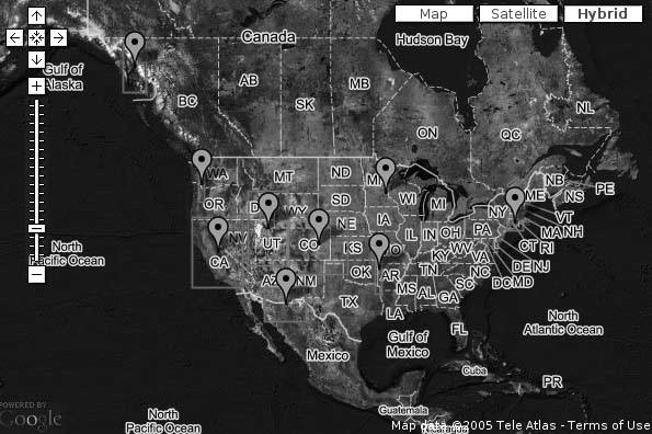
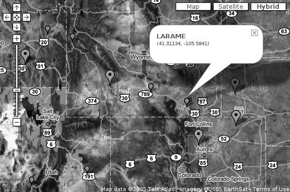
The solution that we eventually hit upon for visualizing all of Rich's travels at once can be seen at http://mappinghacks.com/projects/gmaps/cluster.html, as shown in Figure 7-27. The standard Google Maps marker is used to represent a cluster of points, roughly bounded by the red box around the marker. Clicking on a marker pans and zooms the map to the area covered by that cluster. As you get closer in, more localized clusters appear, eventually resolving into the small Google Ridefinder markers, which represent Rich's individual waypoints. Clicking on one of these smaller markers opens a small info window, showing the name and coordinates of the waypoint, as shown in Figure 7-28 .

Figure 7-27. Clusters of points show the general outlines of Rich's travels

Although this demo has some obvious deficiencies, we think that, to some degree, it does succeed at summarizing the data at high zoom levels, while still allowing exploration of the individual data points. Coming up with a lightweight and reasonably fast solution to this problem took a lot of trial and error! Before we take a look at the code, let's peer down the blind alleys we followed before finally settling on our current implementation.

7.9.2. Choosing the Right Clustering Algorithm

Stepping away from the map for a moment, let's restate the problem: we have a large number of points in a two-dimensional coordinate system, which we want to assign to a much smaller number of clusters, based in some way on their relative proximity to each other. This is a fairly common problem in computational statistics, and several well-documented algorithms already exist.

Figure 7-28. Zooming in causes the clusters to resolve as individual waypoints

 

7.9.2.1. k-means clustering.

The first one we tried was the k-means clustering algorithm, which is one of the most popular clustering algorithms in the literature, on account of its relative simplicity:

1. Select a center point for each of k clusters, where k is a small integer.
2. Assign each data point to the cluster whose center point is closest.
3. After all the data points are assigned, move each cluster's center point to the arithmetic mean of the coordinates of all the points in that cluster, treating each dimension separately.
4. Repeat from Step 2, until the center points stop moving.

The other advantage to k-means clustering, aside from its ease of implementation, is that it is relatively quick, usually completing in less than O(n2) time. The most obvious disadvantage of k-means is that you have to somehow select the value of k ahead of time, but we could try to make an educated guess about that. The primary disadvantage of k-means derives from the ambiguity of Step 1: how, exactly, does one select the initial center points? We found that selecting random points in space led to some clusters never acquiring points at all, while randomly selecting points from the data set as initial centers led to the clusters themselves clumping up, which is something we were trying to avoid. Any attempt to choose k or the initial centers based on the data itself only complicated matters, in a sort of recursive fashion. Also, to top it all off, k-means apparently offers not only no guarantee that a globally optimum clustering will result, but not even any guarantee that a "locally" optimum clustering will result. It looked like we were back to the drawing board.

7.9.2.2. Hierarchical clustering.

The next approach we tried was a series of variations on hierarchical clustering algorithms. Instead of iteratively building clusters from the top down, as k-means does, hierarchical algorithms attempt to cluster the data from the bottom up, instead. A typical hierarchical clustering algorithm works as follows:

1. Assign each point to its own cluster.
2. Calculate the distance from each cluster to every other cluster, either from their respective mean centers, or from the two nearest points from each cluster.
3. Take the two closest clusters and combine them into one cluster.
4. Repeat from Step 2, until you have the right number of clusters, or the clusters are some minimum distance apart from each other, or until you have one big cluster.

By now, you can probably guess that hierarchical clustering presents at least one of the same problems as k-meansnamely, that you have to know somehow when you have enough clusters. Also, though hierarchical clustering can be shown to produce globally optimal results, optimality comes with a cost: hierarchical clustering algorithms are frequently known to run to O(n3) time in the worst case. Although this can be mitigated somewhat by clever use of data structures, such as using a heap to store the list of cluster distances, we found that our best attempt at implementing hierarchical algorithms provided reliable results, but it was, quite frankly, too slow. Polynomial-time algorithms are absolutely fine when n is small, but we wanted an approach that could potentially scale to thousands of points and be able to run dynamically in a reasonable time for an HTTP request. The hierarchical approach apparently just wasn't it for us.

7.9.2.3. Naïve grid-based clustering.

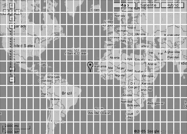
We realized, of course, that we were looking at the problem the wrong way: we didn't need optimal clustering, or mathematically precise clustering, or anything like that. What we were after was some way of consolidating points on a map such that: (a) the markers we display don't wind up overlapping, and (b) we don't show too many markers at once. We can solve requirement (a) by drawing a grid on the map, as shown in Figure 7-29, such that each "cell" in the grid is guaranteed to be at least as large as our marker image when the map is displayed. Next, we take all of the points within any one grid cell and call them a single cluster. For added measure, we can also check each cluster formed this way and see if there are any clusters in the immediately adjacent cells. If there are, we combine them them into a single larger cluster.

Figure 7-29. Assignment of points to clusters based on grid cell membership

By definition, this approach is guaranteed to solve requirement (a), but how likely is it to solve requirement (b)? Initially, we note that the number of clusters we wind up with isn't sensitive to the number of points being clustered, just to their distribution. Let us assume the worst case, where there is at least one point in every potential cell. Let us suppose that a Google Map of the entire world could be as large as 1,024 pixels wide and 768 pixels high, thereby taking up all of an ordinary desktop screen. If the default Google Maps icon is 20 X 34 pixels, then we get a worst case of (1,024 ÷ 20) X (768 ÷ 34) = about 1,156 cells or, at most, 1,196 cells if we round up both sides of the product.

However, since every nine cells will be combined into a supercluster, we wind up with an absolute worst-case maximum of under 150 clusters, which, although not great, isn't horrifying, either. Let's just say that if you have a data set that covers the entire surface of the planet, you might think about using something other than Google Maps to illustrate it. Also, you can see that the algorithm is more sensitive to the size of the grid cells than anything else. At the very least, even if our naïve grid-based algorithm isn't perfect, it can be shown to run in O(n) time, which is an improvement over our earlier experiments.

7.9.3. The Code

The code we developed to test the grid-based clustering algorithm has two parts: first, a CGI script written in Perl runs on the server side, which filters a file of waypoints for those points within a given bounding box, clusters those points as described above, and then spits out an XML file describing the clusters; and second, an HTML page on our server contains client-side JavaScript that uses the Google Maps API to fetch the cluster description for the current map view and plot the clusters on the map.

7.9.3.1. The server-side CGI script.

The CGI script itself is only 120 lines of Perl, but we'll just show the highlights here. If you're interested in looking at the full source, you can find it at http://mappinghacks.com/projects/gmaps/cluster-grid.txt.

Much like the Google Maps interface, our script expects a lat/long center point for the map, and a map span, measured in degrees latitude and longitude. Additionally, because the map geometry matters to our calculations, we also expect a width and height for the intended map in pixels. The following Perl code takes care of that:

	my $q = CGI->new;
	my %var = $q->Vars;

	if ($var{ll} and $var{spn}) {
	 my ($lon, $lat) = split( " ", $var{ll} );
	 my ($width, $height) = split( " ", $var{spn} );
	 $bbox = [ $lon - $width/2, $lat - $height/2,
	 $lon + $width/2, $lat + $height/2 ];
	}

	if ($var{size}) {
	 my ($width, $height) = split( " ", $var{size} );
	 $size = [ $width, $height ];
	}

The result is that the $bbox variable contains a reference to an array listing the minimum longitude and latitude, and the maximum longitude and latitude for our map, in that order. The $size variable similarly stores the width and height of the map in pixels. We then pass $bbox to a function that loads the waypoints from a comma-delimited file, keeping only the ones that fit within our bounding box:

	 while () {
	 chomp;
	 my ($lat, $lon, $name) = split /,s+/, $_;
	 push @data, [$lon, $lat, $name]
	 if $lon >= $bbox->[0] and $lon <= $bbox->[2]
	 and $lat >= $bbox->[1] and $lat <= $bbox->[3];
	}

This hack would be more elegant if we parsed the waypoints from a GPX file instead, but we were aiming to simplify the problem as much as possible, from a technical standpoint. The points themselves are returned as a reference to an array of arrays. We then estimate the grid size in degrees, starting with a hard-coded icon size in pixels, as follows:

	my $icon_size = [ 20, 34 ];
	my $grid_x = $icon_size->[0] / $map_size->[0] * ($bbox->[2] - $bbox->[0]);
	my $grid_y = $icon_size->[1] / $map_size->[1] * ($bbox->[3] - $bbox->[1]);

Basically, we divide the width of the marker icon (in pixels) by the width of the entire map (also in pixels), which gives us a proportion of the map that a single marker would cover, in the horizontal dimension. We multiply this fraction by the total span of the map in degrees longitude, to yield the number of degrees longitude that a marker would cover on a map of this size and span. We then perform the same calculation the marker height, map height, and map span in degrees latitude to get the marker height in degrees latitude. By making our grid cells at least this many degrees wide and high, we can guarantee that none of the markers we place on the map will visually overlap each other by much, if at all.

We then call the cluster() function, which takes the bounding box, the grid cell size, and the data points as arguments:

	sub cluster {
	 my ($bbox, $grid, $data) = @_;
	 my %cluster;

	 for my $point (@$data) {
	 my $col = int( ($point->[0] - $bbox->[0]) / $grid->[0] );
	 my $row = int( ($point->[1] - $bbox->[1]) / $grid->[1] );
	 push @{$cluster{"$col,$row"}}, $point;
	 }

These few lines of code actually do all the work of assigning each point to a cluster. We divide the difference between the point's longitude and the western edge of the map by the grid cell size, which, discarding the remainder, gives us the grid column that the point lies within. We follow a parallel calculation to determine the row of the point, counting from south to north. We then push the point on to a hash of arrays that lists the points within each cell. Since we plan to take each cell that contains one or more points as an initial cluster, this hash is simply called %cluster. We're already halfway finished.

The next bit of code is a bit tricker, as it concerns the neighbor analysis that we use to combine adjacent clusters into superclusters. As a heuristic, we assume that the points are already naturally clustered in some way and conclude that the densest of our initial clusters are most likely to be the "centers" of the combined superclusters. We implement this heuristic by sorting the list of clusters we've found, according to the number of points within each one, in descending order:

	my @groups = sort { @{$cluster{$b}} <=> @{$cluster{$a}} } keys %cluster;

We then iterate over the list of clusters, looking at the eight cells immediately adjacent to each one. If any of the adjacent cells also contains a cluster, we add the points from that cluster to our new supercluster and remove the subsumed cluster from our list. Finally, when all is said and done, we return an array of arrays, containing our original points grouped into clusters.

	 for my $group (@groups) {
	 next unless $cluster{$group};
	 my ($col, $row) = split ",", $group;
	 for my $dx (-1 .. 1) {
	 for my $dy (-1 .. 1) {
	 next unless $dx or $dy;
	 $dx += $col; $dy += $row;
	 if (exists $cluster{"$dx,$dy"}) {
	 my $other = delete $cluster{"$dx,$dy"};
	 push @{$cluster{$group}}, @$other;
	 }
	 }
	 }
	 }

	 return [values %cluster];
	}

We won't bore you with the tedious details of generating XML from this data structure; once again, you can refer to the source code online, if you're particularly interested. However, in order to understand how the JavaScript frontend works, it's worth looking at an example output from this script:

As you can see, this document contains enough information to draw each cluster, as well as to allow the UI to zoom directly in on the extents of any one cluster. Finally, any cluster with only one point isn't really a cluster: it's just a point and is treated as such. The JavaScript user interface therefore only needs to be able to pass the map center, span, and size into this script, and then be able to parse the cluster and point descriptions from the XML output.

7.9.3.2. The client-side JavaScript.

Naturally, the JavaScript frontend to this clustering experiment needs to do all the usual things to import the Google Maps API code and set up the map itself. These tasks are already well-covered elsewhere in this book, and, of course, you can always View Source on the demo page, if you're interested in the details. We'll go straight to the loadClusters() function, which calls our CGI script when the page is loaded:

	function loadClusters () {
	 var request = GXmlHttp.create();
	 var center = map.getCenterLatLng();
	 var span = map.getSpanLatLng();
	 var url = "http://mappinghacks.com/projects/gmaps/cluster-grid.cgi?"
	 url += "ll=" + center.x + "+" + center.y
	 + "&spn=" + span.width + "+" + span.height
	 + "&size=" + map.mapSize.width + "+" + map.mapSize.height;

	 request.open("GET", url, true);
	 request.onreadystatechange = function() {
	 if (request.readyState == 4)
	 showOverlays(request.responseXML);
	 };
	}

This code initiates a GXmlHttp request in the usual way, passing in the map center, span, and size. The map.mapSize property used here is undocumented in the Google Maps API, but you could almost certainly use the DOM API to find out the width and height styles of the map div element instead. When the HTTP request returns, the parsed XML document is passed to the showOverlays() function, which is shown below:

	function showOverlays (xml) {
	 map.clearOverlays();
	 var cluster = xml.documentElement.getElementsByTagName("cluster");
	 for (var i = 0; i < cluster.length; i++) {
	 showCluster( cluster[i] );
	 }
	 var point = xml.documentElement.getElementsByTagName("point");
	 for (var i = 0; i < point.length; i++) {
	 showPoint( point[i] );
	 }
	}

The showOverlays() function clears the map of its existing overlays and then uses the getElementsByTagName() method from the Document Object Model API to extract each cluster and point element from the XML document, passing them one by one to the appropriate rendering function. The showPoint() function doesn't do anything more exciting than put a marker on the map in the appropriate place and bind an info window popup to the click event. Let's look at the showCluster() function, instead, because that's where most of the excitement really is:

	 function showCluster (elem) {
	 var point = new GPoint(parseFloat(elem.getAttribute("lon")),
	 parseFloat(elem.getAttribute("lat")));
	 var width = parseFloat(elem.getAttribute("width")),
	 height = parseFloat(elem.getAttribute("height")),
	 count = parseInt(elem.getAttribute("count"));

	 var marker = new GMarker(point);

The showCluster() function parses the various attributes out of the cluster element and uses the latitude and longitude to create a new marker. So far, no surprises. The action that we bind to that marker's click event is much more interesting:

	 GEvent.addListener(marker, "click", function() {
	 var span = new GSize(width * 1.1, height * 1.1);
	 // undocumented: http://xrl.us/getLowestZoomLevel
	 var zoom = map.spec.getLowestZoomLevel(point, span, map.
	viewSize);

	 loadClusters();
	 map.centerAndZoom(point, zoom);
	 });

Instead of binding an info window to the click event on the marker, we bind an anonymous function that calculates the center point and span of the cluster, augmenting the span by 10% in each dimension, so that all of our points are well within the map view and not hiding out at the edges of the map. Next, we use the method described in "Find the Right Zoom Level" [Hack #58] to calculate the best zoom level for viewing the entire cluster. The anonymous function then calls loadClusters() to kick off a request for the new set of clusters and points for that map view, and then pans and zooms the map to that view.

The finale of the showCluster() function gives the cluster some visual clarity, by drawing a rectangular polyline around the extents of the cluster, so that the user can see which part of the map that the cluster covers:

	 var bbox = new GPolyline(
	 [new GPoint(point.x - width/2, point.y - height/2),
	 new GPoint(point.x - width/2, point.y + height/2),
	 new GPoint(point.x + width/2, point.y + height/2),
	 new GPoint(point.x + width/2, point.y - height/2),
	 new GPoint(point.x - width/2, point.y - height/2)],
	 'ff0000', 2, .80);

	 map.addOverlay(marker);
	 map.addOverlay(bbox);
	}

The user can zoom into a cluster by clicking on it, but what if she wants to zoom back out? A single event handler takes care of refreshing the map display when the user zooms in or out [Hack #60].

	GEvent.addListener(map, "zoom", loadClusters);

 

7.9.4. Conclusion

We've seen here that there can be viable solutions to the vexing problem of what to do when you have too many points to show on a map. We've also seen that some traditional clustering algorithms may be inadequate for certain tasks of practical digital cartography and that a more customized approach, using grid-based clustering, can yield pretty good results. There's no doubt that this method isn't perfect, though, and we'd really like to see it improved upon. If you do use this technique as an inspiration for your own projects, please let us know!

7.9.5. See Also

• Wikipedia on clustering algorithms: http://en.wikipedia.org/wiki/Data_clustering
• "Find the Right Zoom Level" [Hack #58]
• "Show Lots of StuffQuickly" [Hack #59]
• "Make Things Happen When the Map Moves" [Hack #60]