IGRP
Like RIP, the Interior Gateway Routing Protocol is a distance-vector routing protocol. Today, IGRP has been superseded by Enhanced IGRP (EIGRP), which has many new features and is covered later in this chapter. The two protocols are fundamentally similar, configuration-wise, and this section serves as an introduction for both.
IGRP and EIGRP have a compound metric that takes into account several factors, such as link bandwidth and latency. As such, IGRP is superior to RIP, which takes into account only the hop count, and RIPv2, which uses both hop count and bandwidth. In addition to the compound metric, which allows better route selection, IGRP tends to have better convergence times, meaning that routing stabilizes more quickly after a network disruption. In addition, although it is more difficult to configure than RIP, configuration is still relatively easy.
The biggest drawback of IGRP and EIGRP is that they are proprietary, which means they are implemented only by Cisco routers. If all you have on your network are Cisco devices, using IGRP is not a problem. However, if you have a multivendor environment, you'll be forced to use multiple routing protocols or to agree on a protocol (such as RIP or OSPF) that is supported by all your vendors. Another disadvantage is that IGRP (like RIP) broadcasts the entire routing table, which can consume a lot of network bandwidth. In addition, like RIP, IGRP does not support VLSM. If you use VLSMand you probably shouldyou need to use EIGRP.
9.2.1. Basic IGRP Configuration
For this example, we will reuse the network diagram in Figure 9-1. We want to enable IGRP on Router 1 and Router 2. We'll add the bandwidth command on the serial interfaces because IGRP uses bandwidth for the route metric calculation. The bandwidth command is necessary on the serial interfaces because the router is unable to determine a default bandwidth for them. The Ethernet interface does not need a bandwidth command since the router will supply a reasonable default.
The IGRP commands for Router 1 look like this:
interface Ethernet0
 ip address 172.16.1.1 255.255.255.0
!
interface Serial0
 bandwidth 125
 ip address 192.168.3.1 255.255.255.0
!
interface Serial1
 bandwidth 125
 ip address 192.168.1.1 255.255.255.0
!
router igrp 101
 network 172.16.0.0
 network 192.168.1.0
 network 192.168.3.0
For Router 2, they look like this:
interface Ethernet0
 ip address 172.17.1.1 255.255.255.0
!
interface Serial0
 bandwidth 125
 ip address 192.168.1.2 255.255.255.0
!
interface Serial1
 bandwidth 125
 ip address 192.168.2.1 255.255.255.0
!
router igrp 101
 network 172.17.0.0
 network 192.168.1.0
 network 192.168.2.0
And for Router 3, they look like this:
interface Ethernet0
 ip address 172.18.1.1 255.255.255.0
!
interface Serial0
 bandwidth 125
 ip address 192.168.2.2 255.255.255.0
!
interface Serial1
 bandwidth 125
 ip address 192.168.3.2 255.255.255.0
!
router igrp 101
 network 172.18.0.0
 network 192.168.2.0
 network 192.168.3.0
These commands configure IGRP on the proper networks with a local-AS number of 101. The local-AS number is essentially a process number that serves to identify the routers that will exchange routing information. The actual value you pick is immaterial, as long as all the routers running IGRP on the network use the same value. If they do not, they won't share routing information.
Let's run show ip route and send a few pings to make sure everything is running well:
Router1#show ip route
Codes: C - connected, S - static, I - IGRP
, R - RIP, M - mobile, B - BGP
 D - EIGRP, EX - EIGRP external, O - OSPF, IA - OSPF inter area
 N1 - OSPF NSSA external type 1, N2 - OSPF NSSA external type 2
 E1 - OSPF external type 1, E2 - OSPF external type 2, E - EGP
 i - IS-IS, L1 - IS-IS level-1, L2 - IS-IS level-2, * - candidate default
 U - per-user static route, o - ODR

Gateway of last resort is not set

I 172.17.0.0/16 [100/82100] via 192.168.1.2, 00:01:05, Serial1
 172.16.0.0/24 is subnetted, 1 subnets
C 172.16.1.0 is directly connected, Ethernet0
I 172.18.0.0/16 [100/82100] via 192.168.3.2, 00:00:02, Serial0
C 192.168.1.0/24 is directly connected, Serial1
I 192.168.2.0/24 [100/84000] via 192.168.1.2, 00:01:06, Serial1
 [100/84000] via 192.168.3.2, 00:00:02, Serial0
C 192.168.3.0/24 is directly connected, Serial0
From Router 1, ping Router 2's Ethernet interface:
Router1#ping 172.17.1.1

Type escape sequence to abort.
Sending 5, 100-byte ICMP Echos to 172.17.1.1, timeout is 2 seconds:
!!!!!
Success rate is 100 percent (5/5), round-trip min/avg/max = 28/31/32 ms
From Router 1, ping Router 3's Ethernet interface:
Router1#ping 172.18.1.1

Type escape sequence to abort.
Sending 5, 100-byte ICMP Echos to 172.18.1.1, timeout is 2 seconds:
!!!!!
Success rate is 100 percent (5/5), round-trip min/avg/max = 28/31/32 ms
Once again, the ping shows only that a working path exists between two hosts. It is by no means a complete test of our routing configuration.
9.2.1.1. IGRP's metric
Previously, we called the metric used by IGRP a compound metric, which means it uses more than one value to decide which route to use. The factors IGRP uses to calculate a metric are bandwidth, load, delay, and reliability. Before we examine the formula used to compute the metric, you should understand each of the variables:
bandwidth
The speed of the line. The bandwidth of any particular link is a configuration itemit isn't derived from the hardware itself. However, there are defaults for almost all media types except serial links. Ethernet, FDDI, token ring, etc., all have default bandwidth settings. Bandwidth is measured in 1-Kbps units; thus, the bandwidth for an Ethernet link is 10,000 Kbps.
delay
The total delay for the path in 10-microsecond units. To get the delay for the entire route, the delay values for all the route's links are added together and the result is divided by 10.
load
A number between 1 and 255, which is a fraction of 255 that reflects the link's usage. A fully loaded link has the value of 255 (which equals 100%); a link with no load is assigned the value 1, which is the lowest possible value. If the loading were at 50%, the load value would be 128 (128/255).
reliability
Like load, reliability is a fraction of 255, where 255 represents 100% reliability and 1 represents the lowest reliability.
In all its gory detail, the metric equation is:

If K5 is greater than 0, you need to apply this second step:
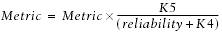
K1 through K5 are constants used to control the equation's behavior. By varying these constants, you can give a higher or lower priority to different variables. By default, K1 and K3 equal 1, and K2, K4, and K5 equal 0. This means that, in effect, the metric calculation is much simpler:
Metric = bandwidth + delay
As with any distance-vector protocol, the route with the smallest metric (think in terms of weight) is the best route for the packet to travel.
Despite all this talk about a compound metric, it's apparent that IGRP's default metric is really quite simple and depends only on the bandwidth and the delay. What's the use of having a great compound metric if you set up the constants so that most of the interesting features of that metric are discarded? Well, it is possible to adapt the metric for use in special situations. The command for changing the constants is meTRic weights tos k1 k2 k3 k4 k5. (The tos is a value that is not used; refer to Chapter 17 for an explanation.)
Making intelligent decisions about how to change the constants is beyond the scope of this book. It's easy to make a change that has side effects you don't want. For example, we could tell the router to use the load factor by setting K2 to 1. However, in most networks, this change would have a serious side effect. A link's load can increase and decrease fairly quickly. Each change to the load would cause the link's metric to change and a route update to occur. As metrics change, routing updates and broadcasts also change. This can be an important fact when dealing with a state-driven protocol such as EIGRP. For example, using load and reliability might cause unstable routing tables, because they tend to oscillate based on small changes in traffic volume.
There may be situations in which you want this behavior, but on most networks, you don't want to send routing updates more frequently than necessary. Whatever the reasons, changing the K values should be done cautiously, if at all. It's best not to change the metrics.
9.2.1.2. Packet size
IGRP also keeps track of the Maximum Transmission Unit (MTU) on every path it knows about. The MTU is the largest packet that can be sent without fragmentation. The MTU for an entire route is the smallest MTU of any of the links in that route.
9.2.1.3. Modifying the range of the network
Like RIP, IGRP also keeps track of hop counts, although they aren't used in computing the routing metric. Hop counts are used to decide when a network has become unreachable. By default, the maximum hop count is 100; however, you can set it to be as high as 255 using the command meTRic maximum hops:
router igrp 101
 metric maximum-hops 200
Note that the maximum hop count of IGRP allows it to support much larger networks than RIP, which supports only 15 hops as a maximum.
9.2.1.4. IGRP's load balancing
IGRP performs either equal-cost load balancing or unequal-cost load balancing. Load balancing means that IGRP distributes the network traffic load across more than one link. However, IGRP (and EIGRP) do load balancing on a session-oriented basis. Load balancing is not packet-oriented; therefore, once a session has been started with a host somewhere on the network, all packets in that session will be sent through the same interface.
In equal-cost load balancing , a router can have up to four routes to a particular destination, as long as all the routes have the same (equal) metric. For example, let's assume that a route has a metric of 9,000, and another route to the same destination comes along. The new route is added to the route table, but it is used for load balancing only if its metric is also 9,000. If the metric of the new route is less than 9,000, it will be used for all the traffic, and the original route won't be used. On the other hand, if the new route has a metric greater than 9,000, the router will know of its existence but won't use it to handle any traffic.
Unequal-cost load balancing requires the use of a metric multiplier, which is called a variance . The variance allows other routes to be added to the routing table even if their metrics are not equal. Before any new route is added to the table, however, two rules must be met:
- The new router's metric to the destination must be less than our router's current metric to the destination. Or more simply, the new router must be closer than our router.
- The variance multiplied by our router's metric must be equal to or greater than the new route. Or more simply, our route multiplied by some number (variance) must be larger than the new route's metric. So we are willing to accept an alternate route if its metric is within some fraction of our current metric.
As with equal-cost load balancing , the router keeps up to four routes to a destination in its routing table. If more than four routes are available, only the best four are used. If you understood the two rules, you realized that equal-cost load balancing is nothing more than unequal-cost load balancing with a variance of 1, which is the default value. So the router performs equal-cost load balancing by default; you can set the variance to another value using the variance command. Increasing the variance allows traffic to be distributed over links with unequal metrics. This means that if our primary link is becoming loaded, we can distribute some of the load across the otherwise unused, slower links.
These rules are admittedly confusing; it will help to look at an example. Figure 9-2 shows a simple network with three routers. Our router is Router 1, and we are interested in routes to Router 2. Normally, we would send all our traffic over Route 1, which is a T1 link with a metric of 8,000. Of the routes we have available, this route is clearly the best. But let's see what happens with unequal-cost load balancing. Imagine that the variance is 4. Now notice that Router 3 has a route to Router 2 that is also a T1 link with a metric of 8,000. So Router 3's route to Router 2 is as good as ours, thus meeting the first of the two criteria. Furthermore, the total metric for a route from Router 1 to Router 2 via Router 3 is 11,000. That isn't as good as ours, but it is better than our metric times the variance (11,000 is less than 8,000 x 4). So if our variance is 4, we will add this second route via Router 3 to our routing table and start using it to carry traffic.
Figure 9-2. An example of unequal-cost load balancing
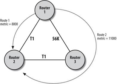
While we used a variance of 4 to illustrate our example, it's not advisable to use a variance of more than 1.5, because the slower link will have a much larger latency due to transmission time. For example, a 56k link takes .21 seconds to transmit a 1,500-byte packet, and a T1 takes .001 seconds.
With unequal-cost load balancing, traffic is distributed across all possible routes in the route table (there are four maximum routes). We can change this behavior so that the best route is used all the time, and extra routes are used only when the best route becomes unavailable. The command that controls this feature is TRaffic-share, which by default is set to balanced. In the following example, we change traffic sharing to min (minimum), which sends all traffic to the route with the best metric. We also specify a variance of 2:
router igrp 100
 network 10.0.0.0
 variance 2
 traffic-share min across-interfaces
The advantage of this configuration is that the extra routes are held in the routing table and are immediately available if the primary route goes down, but there is no attempt at load balancing between routes of unequal quality.
You can perform load balancing on a per-packet basis by using process switching, which is discussed in Chapter 8. Process switching is more CPU-intensive but may be a better solution in some applications.
9.2.2. Redistributing Other Protocols into IGRP
When redistributing RIP into IGRP , you must define a default metric that tells IGRP how to assign metrics for the routes it learns from RIP. The following example uses the redistribute command and the default-metric command:
! Define the IGRP routing process
router igrp 100
 network 10.0.0.0
 redistribute rip
 default-metric 10000 100 255 1 1500
! Define the RIP process
router rip
 network 192.168.1.0
The default-metric command is required for redistributing most nonstatic routes. In this example, we specify the values that are the input for IGRP's metric computation. The values indicate bandwidth (10,000, which is 10,000 Kbps), delay (in units of tens of microseconds100 equals a delay of 1 millisecond), reliability (1 to 255), load (1 to 255), and the MTU (1500 bytes). These are all reasonable values for a 10 Mbps Ethernet. A reasonable default metric for a serial link might be:
default-metric 1000 100 250 100 1500
Getting Started
- Getting Started
- IOS User Modes
- Command-Line Completion
- Get to Know the Question Mark
- Command-Line Editing Keys
- Pausing Output
- show Commands
IOS Images and Configuration Files
- IOS Images and Configuration Files
- IOS Image Filenames
- The New Cisco IOS Packaging Model
- Loading Image Files Through the Network
- Using the IOS Filesystem for Images
- The Routers Configuration
- Loading Configuration Files
Basic Router Configuration
- Basic Router Configuration
- Setting the Router Name
- Setting the System Prompt
- Configuration Comments
- The Enable Password
- Mapping Hostnames to IP Addresses
- Setting the Routers Time
- Enabling SNMP
- Cisco Discovery Protocol
- System Banners
Line Commands
- Line Commands
- The line Command
- The Console Port
- Virtual Terminals (VTYs)
- Asynchronous Ports (TTYs)
- The Auxiliary (AUX) Port
- show line
- Reverse Telnet
- Common Configuration Items
Interface Commands
- Interface Commands
- Naming and Numbering Interfaces
- Basic Interface Configuration Commands
- The Loopback Interface
- The Null Interface
- Ethernet, Fast Ethernet, and Gigabit Ethernet Interfaces
- Token Ring Interfaces
- ISDN Interfaces
- Serial Interfaces
- Asynchronous Interfaces
- Interface show Commands
Networking Technologies
Access Lists
IP Routing Topics
- IP Routing Topics
- Autonomous System (AS) Numbers
- Interior and Exterior Gateway Protocols
- Distance-Vector and Link-State Routing Protocols
- Static Routes
- Split Horizon
- Passive Interfaces
- Fast Switching and Process Switching
Interior Routing Protocols
Border Gateway Protocol
- Border Gateway Protocol
- Introduction to BGP
- A Simple BGP Configuration
- Route Filtering
- An Advanced BGP Configuration
- Neighbor Authentication
- Peer Groups
- Route Reflectors
- BGP Confederacies
- BGP TTL Security
Quality of Service
- Quality of Service
- Marking
- Older Queuing Methods
- Modern IOS QoS Tools
- Congestion Avoidance
- Traffic Policing
- Traffic Shaping
- AutoQoS
- QoS Device Manager
Dial-on-Demand Routing
- Dial-on-Demand Routing
- Configuring a Simple DDR Connection
- Sample Legacy DDR Configurations
- Dialer Interfaces (Dialer Profiles)
- Multilink PPP
- Snapshot DDR
Specialized Networking Topics
- Specialized Networking Topics
- Bridging
- Hot Standby Routing Protocol (HSRP)
- Network Address Translation (NAT)
- Tunnels
- Encrypted Tunnels
- Multicast Routing
- Multiprotocol Label Switching (MPLS)
Switches and VLANs
- Switches and VLANs
- Switch Terminology
- IOS on Switches
- Basic Switch Configuration
- Trunking
- Switch Monitor Port for IDS or Sniffers
- Troubleshooting Switches
Router Security
- Router Security
- Securing Enable Mode Access
- Routine Security Measures
- Restricting Access to Your Router
Troubleshooting and Logging
Quick Reference
Appendix A Network Basics
Index
EAN: 2147483647
Pages: 1031
