LOW-PASS FIR FILTER DESIGN
OK, instead of just accepting a given set of FIR filter coefficients and analyzing their frequency response, let's reverse the process and design our own low-pass FIR filter. The design procedure starts with the determination of a desired frequency response followed by calculating the filter coefficients that will give us that response. There are two predominant techniques used to design FIR filters: the window method and the so-called optimum method. Let's discuss them in that order.
5.3.1 Window Design Method
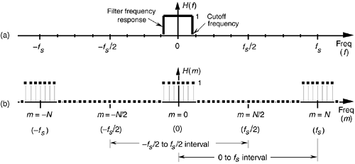
The window method of FIR filter design (also called the Fourier series method) begins with our deciding what frequency response we want for our low-pass filter. We can start by considering a continuous low-pass filter, and simulating that filter with a digital filter. We'll define the continuous frequency response H(f) to be ideal, i.e., a low-pass filter with unity gain at low frequencies and zero gain (infinite attenuation) beyond some cutoff frequency, as shown in Figure 5-14(a). Representing this H(f) response by a discrete frequency response is straightforward enough because the idea of a discrete frequency response is essentially the same as a continuous frequency response—with one important difference. As described in Sections 2.2 and 3.13, discrete frequency-domain representations are always periodic with the period being the sample rate fs. The discrete representation of our ideal, continuous low-pass filter H(f) is the periodic response H(m) depicted by the frequency-domain samples in Figure 5-14(b).
Figure 5-14. Low-pass filter frequency responses: (a) continuous frequency response H(f); (b) periodic, discrete frequency response H(m).
We have two ways to determine our low-pass filter's time-domain coefficients. The first way is algebraic:
- Develop an expression for the discrete frequency response H(m).
- Apply that expression to the inverse DFT equation to get the time domain h(k).
- Evaluate that h(k) expression as a function of time index k.
The second method is to define the individual frequency-domain samples representing H(m) and then have a software routine perform the inverse DFT of those samples, giving us the FIR filter coefficients. In either method, we need only define the periodic H(m) over a single period of fs Hz. As it turns out, defining H(m) in Figure 5-14(b) over the frequency span –fs/2 to fs/2 is the easiest form to analyze algebraically, and defining H(m) over the frequency span 0 to fs is the best representation if we use the inverse DFT to obtain our filter's coefficients. Let's try both methods to determine the filter's time-domain coefficients.
In the algebraic method, we can define an arbitrary discrete frequency response H(m) using N samples to cover the –fs/2 to fs/2 frequency range and establish K unity-valued samples for the passband of our low-pass filter as shown in Figure 5-15. To determine h(k) algebraically we need to take the inverse DFT of H(m) in the form of

Figure 5-15. Arbitrary, discrete low-pass FIR filter frequency response defined over N frequency-domain samples covering the frequency range of fs Hz.

where our time-domain index is k. The solution to Eq. (5-9), derived in Section 3.13 as Eq. (3-59), is repeated here as
Equation 5-10

If we evaluate Eq. (5-10) as a function of k, we get the sequence shown in Figure 5-16 taking the form of the classic sin(x)/x function. By reviewing the material in Section 3.13, it's easy to see the great deal of algebraic manipulation required to arrive at Eq. (5-10) from Eq. (5-9). So much algebra, in fact, with its many opportunities for making errors, that digital filter designers like to avoid evaluating Eq. (5-9) algebraically. They prefer to use software routines to perform inverse DFTs (in the form of an inverse FFT) to determine h(k), and so will we.
Figure 5-16. Time-domain h(k) coefficients obtained by evaluating Eq. (5-10).

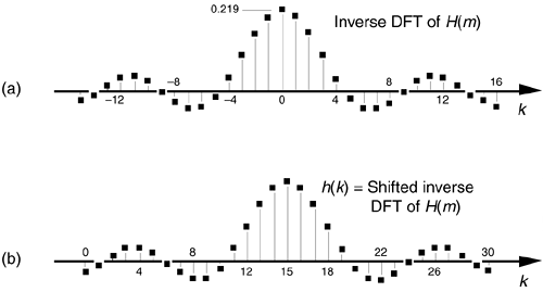
We can demonstrate the software inverse DFT method of FIR filter design with an example. Let's say we need to design a low-pass FIR filter simulating the continuous frequency response shown in Figure 5-17(a). The discrete representation of the filter's frequency response H(m) is shown in Figure 5-17(b), where we've used N = 32 points to represent the frequency-domain variable H(f). Because it's equivalent to Figure 5-17(b) but avoids the negative values of the frequency index m, we represent the discrete frequency samples over the range 0 to fs in Figure 5-17(c), as opposed to the –fs/2 to +fs/2 range in Figure 5-17(b). OK, we're almost there. Using a 32-point inverse FFT to implement a 32-point inverse DFT of the H(m) sequence in Figure 5-17(c), we get the 32 h(k) values depicted by the dots from k = –15 to k = 16 in Figure 5-18(a).[] We have one more step to perform. Because we want our final 31-tap h(k) filter coefficients to be symmetrical with their peak value in the center of the coefficient sample set, we drop the k = 16 sample and shift the k index to the left from Figure 5-18(a), giving us the desired sin(x)/x form of h(k) as shown in Figure 5-18(b). This shift of the index k will not change the frequency magnitude response of our FIR filter. (Remember from our discussion of the DFT Shifting Theorem in Section 3.6 that a shift in the time domain manifests itself only as a linear phase shift in the frequency domain with no change in the frequency domain magnitude.) The sequence in Figure 5-18(b), then, is now the coefficients we use in the convolution process of Figure 5-5 to implement a low-pass FIR filter.
[] If you want to use this FIR design method but only have a forward FFT software routine available, Section 13.6 shows a slick way to perform an inverse FFT with the forward FFT algorithm.
Figure 5-17. An ideal low-pass filter: (a) continuous frequency response H(f); (b) discrete response H(m) over the range of –fs/2 to fs/2 Hz; (c) discrete response H(m) over the range 0 to fs Hz.
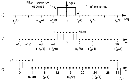
Figure 5-18. Inverse DFT of the discrete response in Figure 5-17(c): (a) normal inverse DFT indexing for k; (b) symmetrical coefficients used for a 31-tap low-pass FIR filter.
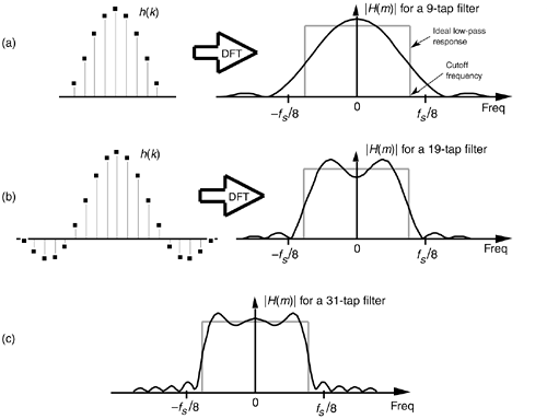
It's important to demonstrate that the more h(k) terms we use as filter coefficients, the closer we'll approximate our ideal low-pass filter response. Let's be conservative, just use the center nine h(k) coefficients, and see what our filter response looks like. Again, our filter's magnitude response in this case will be the DFT of those nine coefficients as shown on the right side of Figure 5-19(a). The ideal filter's frequency response is also shown for reference as the dashed curve. (To show the details of its shape, we've used a continuous curve for |H(m)| in Figure 5-19(a), but we have to remember that |H(m)| is really a sequence of discrete values.) Notice that using nine coefficients gives us a low-pass filter, but it's certainly far from ideal. Using more coefficients to improve our situation, Figure 5-19(b) shows 19 coefficients and their corresponding frequency magnitude response that is beginning to look more like our desired rectangular response. Notice that magnitude fluctuations, or ripples, are evident in the passband of our H(m) filter response. Continuing, using all 31 of the h(k) values for our filter coefficients results in the frequency response in Figure 5-19(c). Our filter's response is getting better (approaching the ideal), but those conspicuous passband magnitude ripples are still present.
Figure 5-19. Coefficients and frequency responses of three low-pass filters: (a) 9-tap FIR filter; (b) a 19-tap FIR filter; (c) frequency response of the full 31-tap FIR filter.
It's important that we understand why those passband ripples are in the low-pass FIR filter response in Figure 5-19. Recall the above discussion of convolving the 5-tap averaging filter coefficients, or impulse response, with an input data sequence to obtain the averager's output. We established that convolution in the time domain is equivalent to multiplication in the frequency domain, that we symbolized with Eq. (5-8), and repeat it here as
Equation 5-11

This association between convolution in the time-domain and multiplication in the frequency domain, sketched in Figure 5-7, indicates that, if two time-domain sequences h(k) and x(n) have DFTs of H(m) and X(m), respectively, then the DFT of h(k) * x(n) is H(m) · X(m). No restrictions whatsoever need be placed on what the time-domain sequences h(k) and x(n) in Eq. (5-11) actually represent. As detailed later in Section 5.9, convolution in one domain is equivalent to multiplication in the other domain, allowing us to state that multiplication in the time domain is equivalent to convolution in the frequency domain, or
Equation 5-12

Now we're ready to understand why the magnitude ripples are present in Figure 5-19.
Rewriting Eq. (5-12) and replacing the h(k) and x(n) expressions with h (k) and w(k), respectively,
Equation 5-13

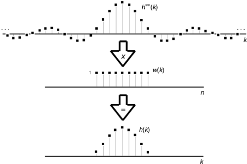
Let's say that h (k) represents an infinitely long sin(x)/x sequence of ideal low-pass FIR filter coefficients and that w(k) represents a window sequence that we use to truncate the sin(x)/x terms as shown in Figure 5-20. Thus, the w(k) sequence is a finite-length set of unity values and its DFT is W(m). The length of w(k) is merely the number of coefficients, or taps, we intend to use to implement our low-pass FIR filter. With h
 (k) defined as such, the product h
 (k) · w(k) represents the truncated set of filter coefficients h(k) in Figures 5-19(a) and 5-19(b). So, from Eq. (5-13), the FIR filter's true frequency response H(m) is the convolution
Equation 5-14

Figure 5-20. Infinite h (k) sequence windowed by w(k) to define the final filter coefficients h(k).
We depict this convolution in Figure 5-21 where, to keep the figure from being so busy, we show H (m) (the DFT of the h
 (k) coefficients) as the dashed rectangle. Keep in mind that it's really a sequence of constant-amplitude sample values.
Figure 5-21. Convolution W(m)*H (m): (a) unshifted W(m) and H
 (m); (b) shift of W(m) leading to ripples within H(m)'s positive frequency passband; (c) shift of W(m) causing response roll-off near H(m)'s positive cutoff frequency; (d) shift of W(m) causing ripples beyond H(m)'s positive cutoff frequency.
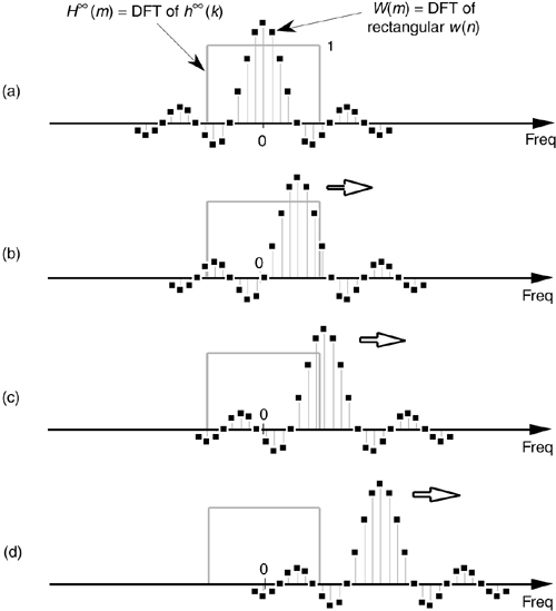
Let's look at Figure 5-21(a) very carefully to see why all three |H(m)|s exhibit passband ripple in Figure 5-19. We can view a particular sample value of the H(m) = H (m) * W(m) convolution as being the sum of the products of H
 (m) and W(m) for a particular frequency shift of W(m). H
 (m) and the unshifted W(m) are shown in Figure 5-21(a.) With an assumed value of unity for all of H
 (m), a particular H(m) value is now merely the sum of the W(m) samples that overlap the H
 (m) rectangle. So, with a W(m) frequency shift of 0 Hz, the sum of the W(m) samples that overlap the H
 (m) rectangle in Figure 5-21(a) is the value of H(m) at 0 Hz. As W(m) is shifted to the right to give us additional positive frequency H(m) values, we can see that the sum of the positive and negative values of W(m) under the rectangle oscillate during the shifting of W(m). As the convolution shift proceeds, Figure 5-21(b) shows why there are ripples in the passband of H(m)—again, the sum of the positive and negative W(m) samples under the H
 (m) rectangle continue to vary as the W(m) function is shifted. The W(m) frequency shift, indicated in Figure 5-21(c), where the peak of W(m)'s main lobe is now outside the H
 (m) rectangle, corresponds to the frequency where H(m)'s passband begins to roll off. Figure 5-21(d) shows that, as the W(m) shift continues, there will be ripples in H(m) beyond the positive cutoff frequency.[
 ] The point of all of this is that the ripples in H(m) are caused by the sidelobes of W(m).
[
] In Figure 5-21(b), had we started to shift W(m) to the left in order to determine the negative frequency portion of H(m), we would have obtained the mirror image of the positive frequency portion of H(m).
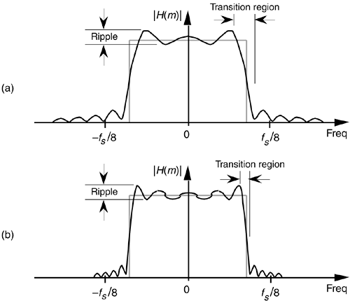
Figure 5-22 helps us answer the question: How many sin(x)/x coefficients do we have to use (or how wide must w(k) be) to get nice sharp falling edges and no ripples in our H(m) passband? The answer is that we can't get there from here. It doesn't matter how many sin(x)/x coefficients (filter taps) we use, there will always be filter passband ripple. As long as w(k) is a finite number of unity values (i.e., a rectangular window of finite width) there will be sidelobe ripples in W(m), and this will induce passband ripples in the final H(m) frequency response. To illustrate that increasing the number of sin(x)/x coefficients doesn't reduce passband ripple, we repeat the 31-tap, low-pass filter response in Figure 5-22(a). The frequency response, using 63 coefficients, is shown in Figure 5-22(b), and the passband ripple remains. We can make the filter's transition region more narrow using additional h(k) filter coefficients, but we cannot eliminate the passband ripple. That ripple, known as Gibbs' phenomenon, manifests itself anytime a function (w(k) in this case) with a instantaneous discontinuity is represented by a Fourier series[6–8]. No finite set of sinusoids will be able to change fast enough to be exactly equal to an instantaneous discontinuity. Another way to state this Gibbs' dilemma is that, no matter how wide our w(k) window is, its DFT of W(m) will always have sidelobe ripples. As shown in Figure 5-22(b), we can use more coefficients by extending the width of the rectangular w(k) to narrow the filter transition region, but a wider w(k) does not eliminate the filter passband ripple nor does it even reduce their peak-to-peak ripple magnitudes, as long as w(k) has sudden discontinuities.
Figure 5-22. Passband ripple and transition regions: (a) for a 31-tap low-pass filter; (b) for a 63-tap low-pass filter.
5.3.2 Windows Used in FIR Filter Design
OK. The good news is that we can minimize FIR passband ripple with window functions the same way we minimized DFT leakage in Section 3.9. Here's how. Looking back at Figure 5-20, by truncating the infinitely long h (k) sequence through multiplication by the rectangular w(k), our final h(k) exhibited ripples in the frequency-domain passband. Figure 5-21 shows us that the passband ripples were caused by W(m)'s sidelobes that, in turn, were caused by the sudden discontinuities from zero to one and one to zero in w(k). If we think of w(k) in Figure 5-20 as a rectangular window, then, it is w(k)'s abrupt amplitude changes that are the source of our filter passband ripple. The window FIR design method is the technique of reducing w(k)'s discontinuities by using window functions other than the rectangular window.
Consider Figure 5-23 to see how a nonrectangular window function can be used to design low-ripple FIR digital filters. Imagine if we replaced Figure 5-20's rectangular w(k) with the Blackman window function whose discrete values are defined as[ ]
]
[
] As we mentioned in Section 3.9, specific expressions for window functions depend on the range of the sample index k. Had we defined k to cover the range –N/2, < k < N/2, for example, the expression for the Blackman window would have a sign change and be w(k) = 0.42 + 0.5cos(2pk/N) + 0.08cos(4pk/N).
Equation 5-15

Figure 5-23. Coefficients and frequency response of a 31-tap Blackman-windowed FIR Filter: (a) defining the windowed filter coefficients h(k); (b) low-ripple 31-tap frequency response; (c) low-ripple 63-tap frequency response.
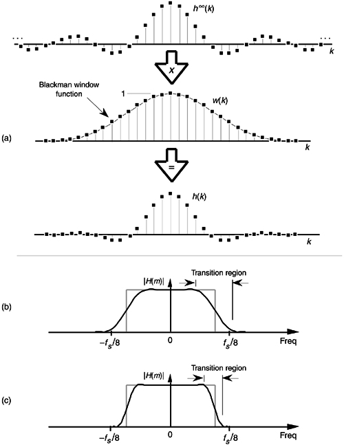
This situation is depicted for N = 31 in Figure 5-23(a), where Eq. (5-15)'s w(k) looks very much like the Hanning window function in Figure 3-17(a). This Blackman window function results in the 31 smoothly tapered h(k) coefficients at the bottom of Figure 5-23(a). Notice two things about the resulting H(m) in Figure 5-23(b). First, the good news. The passband ripples are greatly reduced from those evident in Figure 5-22(a)—so our Blackman window function did its job. Second, the price we paid for reduced passband ripple is a wider H(m) transition region. We can get a steeper filter response roll-off by increasing the number of taps in our FIR filter. Figure 5-23(c) shows the improved frequency response had we used a 63-coefficient Blackman window function for a 63-tap FIR filter. So using a nonrectangular window function reduces passband ripple at the expense of slower passband to stopband roll-off.
A graphical comparison of the frequency responses for the rectangular and Blackman windows is provided in Figure 5-24. (The curves in Figure 5-24 were obtained for the window functions defined by 32 discrete samples, to which 480 zeros were appended, applied to a 512-point DFT.) The sidelobe magnitudes of the Blackman window's |W(m)| are too small to see on a linear scale. We can see those sidelobe details by plotting the two windows' frequency responses on a logarithmic scale and normalizing each plot so that their main lobe peak values are both zero dB. For a given window function, we can get the log magnitude response of WdB(m) by using the expression
Equation 5-16

Figure 5-24. Rectangular vs. Blackman window frequency magnitude responses: (a) |W(m)| on a linear scale; (b) normalized logarithmic scale of WdB(m).

(The |W(0)| term in Eq. (5-16) is the magnitude of W(m) at the peak of the main lobe when m = 0.) Figure 5-24(b) shows us the greatly reduced sidelobe levels of the Blackman window and how that window's main lobe is almost three times as wide as the rectangular window's main lobe.
Of course, we could have used any of the other window functions, discussed in Section 3.9, for our low-pass FIR filter. That's why this FIR filter design technique is called the window design method. We pick a window function and multiply it by the sin(x)/x values from H (m) in Figure 5-23(a) to get our final h(k) filter coefficients. It's that simple. Before we leave the window method of FIR filter design, let's introduce two other interesting window functions.
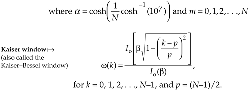
Although the Blackman window and those windows discussed in Section 3.9 are useful in FIR filter design, we have little control over their frequency responses; that is, our only option is to select some window function and accept its corresponding frequency response. Wouldn't it be nice to have more flexibility in trading off, or striking a compromise between, a window's main lobe width and sidelobe levels? Fortunately, there are two popular window functions that give us this opportunity. Called the Chebyshev and the Kaiser window functions, they're defined by the following formidable expressions:
Equation 5-17

Equation 5-18
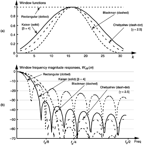
Two typical Chebyshev and Kaiser window functions and their frequency magnitude responses are shown in Figure 5-25. For comparison, the rectangular and Blackman window functions are also shown in that figure. (Again, the curves in Figure 5-25(b) were obtained for window functions defined by 32 discrete samples, with 480 zeros appended, applied to a 512-point DFT.)
Figure 5-25. Typical window functions used with digital filters: (a) window coefficients in the time domain; (b) frequency-domain magnitude responses in dB.
Equation (5-17) was originally based on the analysis of antenna arrays using the mathematics of Chebyshev polynomials[9–11]. Equation (5-18) evolved from Kaiser's approximation of prolate spheroid functions using zeroth-order Bessel functions[12–13]. Don't be intimidated by the complexity of Eqs. (5-17) and (5-18)—at this point, we need not be concerned with the mathematical details of their development. We just need to realize that the control parameters g and b, in Eqs. (5-17) and (5-18), give us control over the windows' main lobe widths and the sidelobe levels.
Let's see how this works for Chebyshev window functions, having four separate values of g, and their frequency responses shown in Figure 5-26. FIR filter designers applying the window method typically use predefined software routines to obtain their Chebyshev window coefficients. Commercial digital signal processing software packages allow the user to specify three things: the window function (Chebyshev in this case), the desired number of coefficients (the number of taps in the FIR filter), and the value of g. Selecting different values for g enables us to adjust the sidelobe levels and see what effect those values have on main lobe width, a capability that we didn't have with the Blackman window or the window functions discussed in Section 3.9. The Chebyshev window function's stopband attenuation, in decibels, is equal to
Equation 5-19

Figure 5-26. Chebyshev window functions for various g values: (a) window coefficients in the time domain; (b) frequency-domain magnitude responses in dB.
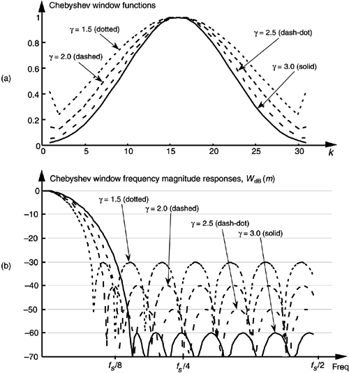
So, for example, if we needed our sidelobe levels to be no greater than –60 dB below the main lobe, we use Eq. (5-19) to establish a g value of 3.0 and let the software generate the Chebyshev window coefficients.[ ]
]
[
] By the way, some digital signal processing software packages require that we specify AttenCheb in decibels instead of g. That way, we don't have to bother using Eq. (5-19) at all.
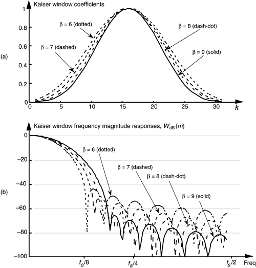
The same process applies to the Kaiser window, as shown in Figure 5-27. Commercial software packages allow us to specify b in Eq. (5-18) and provide us with the associated window coefficients. The curves in Figure 5-27(b), obtained for Kaiser window functions defined by 32 discrete samples, show that we can select the desired sidelobe levels and see what effect this has on the main lobe width.
Figure 5-27. Kaiser window functions for various b values: (a) window coefficients in the time domain; (b) frequency-domain magnitude responses in dB.
Chebyshev or Kaiser, which is the best window to use? It depends on the application. Returning to Figure 5-25(b), notice that, unlike the constant sidelobe peak levels of the Chebyshev window, the Kaiser window's sidelobes decrease with increased frequency. However, the Kaiser sidelobes are higher than the Chebyshev window's sidelobes near the main lobe. Our primary trade-off here is trying to reduce the sidelobe levels without broadening the main lobe too much. Digital filter designers typically experiment with various values of g and b for the Chebyshev and Kaiser windows to get the optimum WdB(m) for a particular application. (For that matter, the Blackman window's very low sidelobe levels outweigh its wide main lobe in many applications.) Different window functions have their own individual advantages and disadvantages for FIR filter design. Regardless of the nonrectangular window function used, they always decrease the FIR filter passband ripple over that of the rectangular window. For the enthusiastic reader, a very thorough discussion of window functions can be found in reference [14].
URL http://proquest.safaribooksonline.com/0131089897/ch05lev1sec3
 |
Amazon |  |
