SIGNAL AMPLITUDE, MAGNITUDE, POWER | Chapter One. Discrete Sequences and Systems

Let's define two important terms that we'll be using throughout this book: amplitude and magnitude. It's not surprising that, to the layman, these terms are typically used interchangeably. When we check our thesaurus, we find that they are synonymous.[] In engineering, however, they mean two different things, and we must keep that difference clear in our discussions. The amplitude of a variable is the measure of how far, and in what direction, that variable differs from zero. Thus, signal amplitudes can be either positive or negative. The time-domain sequences in Figure 1-3 presented the sample value amplitudes of three different waveforms. Notice how some of the individual discrete amplitude values were positive and others were negative.

[] Of course, laymen are "other people." To the engineer, the brain surgeon is the layman. To the brain surgeon, the engineer is the layman.

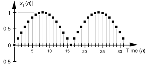
The magnitude of a variable, on the other hand, is the measure of how far, regardless of direction, its quantity differs from zero. So magnitudes are always positive values. Figure 1-4 illustrates how the magnitude of the x1(n) time sequence in Figure 1-3(a) is equal to the amplitude, but with the sign always being positive for the magnitude. We use the modulus symbol (||) to represent the magnitude of x1(n). Occasionally, in the literature of digital signal processing, we'll find the term magnitude referred to as the absolute value.

Figure 1-4. Magnitude samples, |x1(n)|, of the time waveform in Figure 1-3(a).

When we examine signals in the frequency domain, we'll often be interested in the power level of those signals. The power of a signal is proportional to its amplitude (or magnitude) squared. If we assume that the proportionality constant is one, we can express the power of a sequence in the time or frequency domains as

Equation 1-8'

Very often we'll want to know the difference in power levels of two signals in the frequency domain. Because of the squared nature of power, two signals with moderately different amplitudes will have a much larger difference in their relative powers. In Figure 1-3, for example, signal x1(n)'s amplitude is 2.5 times the amplitude of signal x2(n), but its power level is 6.25 that of x2(n)'s power level. This is illustrated in Figure 1-5 where both the amplitude and power of Xsum(m) are shown.

Figure 1-5. Frequency-domain amplitude and frequency-domain power of the xsum(n) time waveform in Figure 1-3(c).

Because of their squared nature, plots of power values often involve showing both very large and very small values on the same graph. To make these plots easier to generate and evaluate, practitioners usually employ the decibel scale as described in Appendix E.

URL http://proquest.safaribooksonline.com/0131089897/ch01lev1sec2