DFT LEAKAGE
Hold on to your seat now. Here's where the DFT starts to get really interesting. The two previous DFT examples gave us correct results because the input x(n) sequences were very carefully chosen sinusoids. As it turns out, the DFT of sampled real-world signals provides frequency-domain results that can be misleading. A characteristic, known as leakage, causes our DFT results to be only an approximation of the true spectra of the original input signals prior to digital sampling. Although there are ways to minimize leakage, we can't eliminate it entirely. Thus, we need to understand exactly what effect it has on our DFT results.
Let's start from the beginning. DFTs are constrained to operate on a finite set of N input values sampled at a sample rate of fs, to produce an N-point transform whose discrete outputs are associated with the individual analytical frequencies fanalysis(m), with
Equation (3-24), illustrated in DFT Example 1, may not seem like a problem, but it is. The DFT produces correct results only when the input data sequence contains energy precisely at the analysis frequencies given in Eq. (3-24), at integral multiples of our fundamental frequency fs/N. If the input has a signal component at some intermediate frequency between our analytical frequencies of mfs/N, say 1.5fs/N, this input signal will show up to some degree in all of the N output analysis frequencies of our DFT! (We typically say that input signal energy shows up in all of the DFT's output bins, and we'll see, in a moment, why the phrase "output bins" is appropriate.) Let's understand the significance of this problem with another DFT example.
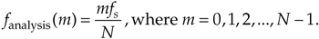
Assume we're taking a 64-point DFT of the sequence indicated by the dots in Figure 3-7(a). The sequence is a sinewave with exactly three cycles contained in our N = 64 samples. Figure 3-7(b) shows the first half of the DFT of the input sequence and indicates that the sequence has an average value of zero (X(0) = 0) and no signal components at any frequency other than the m = 3 frequency. No surprises so far. Figure 3-7(a) also shows, for example, the m = 4 sinewave analysis frequency, superimposed over the input sequence, to remind us that the analytical frequencies always have an integral number of cycles over our total sample interval of 64 points. The sum of the products of the input sequence and the m = 4 analysis frequency is zero. (Or we can say, the correlation of the input sequence and the m = 4 analysis frequency is zero.) The sum of the products of this particular three-cycle input sequence and any analysis frequency other than m = 3 is zero. Continuing with our leakage example, the dots in Figure 3-8(a) show an input sequence having 3.4 cycles over our N = 64 samples. Because the input sequence does not have an integral number of cycles over our 64-sample interval, input energy has leaked into all the other DFT output bins as shown in Figure 3-8(b).
Figure 3-7. 64-point DFT: (a) input sequence of three cycles and the m = 4 analysis frequency sinusoid; (b) DFT output magnitude.
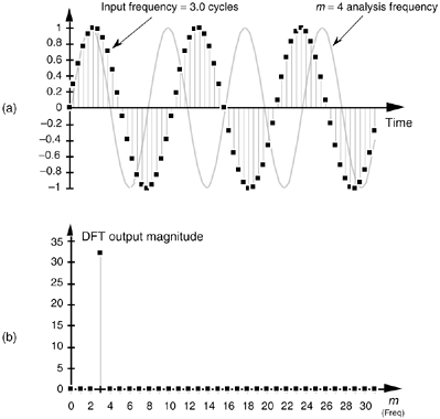
Figure 3-8. 64-point DFT: (a) 3.4 cycles input sequence and the m = 4 analysis frequency sinusoid; (b) DFT output magnitude.
The m = 4 bin, for example, is not zero because the sum of the products of the input sequence and the m = 4 analysis frequency is no longer zero. This is leakage—it causes any input signal whose frequency is not exactly at a DFT bin center to leak into all of the other DFT output bins. Moreover, leakage is an unavoidable fact of life when we perform the DFT on real-world finite-length time sequences.
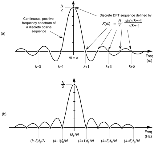
Now, as the English philosopher Douglas Adams would say, "Don't panic." Let's take a quick look at the cause of leakage to learn how to predict and minimize its unpleasant effects. To understand the effects of leakage, we need to know the amplitude response of a DFT when the DFT's input is an arbitrary, real sinusoid. Although Sections 3.14 and 3.15 discuss this issue in detail, for our purposes, here, we'll just say that, for a real cosine input having k cycles in the N-point input time sequence, the amplitude response of an N-point DFT bin in terms of the bin index m is approximated by the sinc function
Equation 3-25
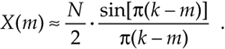
We'll use Eq. (3-25), illustrated in Figure 3-9(a), to help us determine how much leakage occurs in DFTs. We can think of the curve in Figure 3-9(a), comprising a main lobe and periodic peaks and valleys known as sidelobes, as the continuous positive spectrum of an N-point, real cosine time sequence having k complete cycles in the N-point input time interval. The DFT's outputs are discrete samples that reside on the curves in Figure 3-9; that is, our DFT output will be a sampled version of the continuous spectrum. (We show the DFT's magnitude response to a real input in terms of frequency (Hz) in Figure 3-9(b).) When the DFT's input sequence has exactly an integral k number of cycles (centered exactly in the m = k bin), no leakage occurs, as in Figure 3-9, because when the angle in the numerator of Eq. (3-25) is a nonzero integral multiple of p, the sine of that angle is zero.
Figure 3-9. DFT positive frequency response due to an N-point input sequence containing k cycles of a real cosine: (a) amplitude response as a function of bin index m; (b) magnitude response as a function of frequency in Hz.
By way of example, we can illustrate again what happens when the input frequency k is not located at a bin center. Assume that a real 8-kHz sinusoid, having unity amplitude, has been sampled at a rate of fs = 32,000 samples/s. If we take a 32-point DFT of the samples, the DFT's frequency resolution, or bin spacing, is fs/N = 32,000/32 Hz = 1.0 kHz. We can predict the DFT's magnitude response by centering the input sinusoid's spectral curve at the positive frequency of 8 kHz, as shown in Figure 3-10(a). The dots show the DFT's output bin magnitudes.
Figure 3-10. DFT bin positive frequency responses: (a) DFT input frequency = 8.0 kHz; (b) DFT input frequency = 8.5 kHz; (c) DFT input frequency = 8.75 kHz.
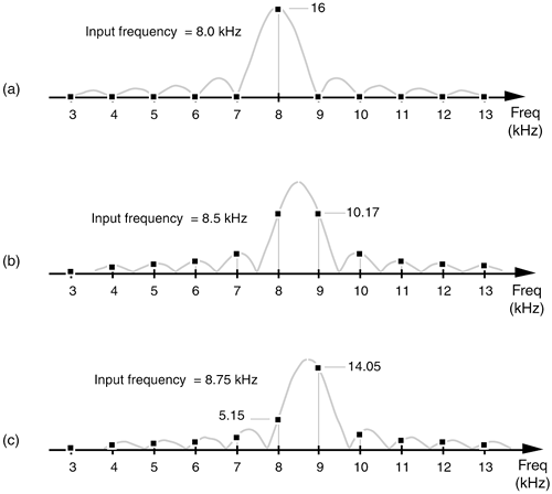
Again, here's the important point to remember: the DFT output is a sampled version of the continuous spectral curve in Figure 3-10(a). Those sampled values in the frequency-domain, located at mfs/N, are the dots in Figure 3-10(a). Because the input signal frequency is exactly at a DFT bin center, the DFT results have only one nonzero value. Stated in another way, when an input sinusoid has an integral number of cycles over N time-domain input sample values, the DFT outputs reside on the continuous spectrum at its peak and exactly at the curve's zero crossing points. From Eq. (3-25) we know the peak output magnitude is 32/2 = 16. (If the real input sinusoid had an amplitude of 2, the peak of the response curve would be 2 · 32/2, or 32.) Figure 3-10(b) illustrates DFT leakage where the input frequency is 8.5 kHz, and we see that the frequency-domain sampling results in nonzero magnitudes for all DFT output bins. An 8.75-kHz input sinusoid would result in the leaky DFT output shown in Figure 3-10(c). If we're sitting at a computer studying leakage by plotting the magnitude of DFT output values, of course, we'll get the dots in Figure 3-10 and won't see the continuous spectral curves.
At this point, the attentive reader should be thinking: "If the continuous spectra that we're sampling are symmetrical, why does the DFT output in Figure 3-8(b) look so asymmetrical?" In Figure 3-8(b), the bins to the right of the third bin are decreasing in amplitude faster than the bins to the left of the third bin. "And another thing, evaluating the continuous spectrum's X(mfs) function at an abscissa value of 0.4 gives a magnitude scale factor of 0.75. Applying this factor to the DFT's maximum possible peak magnitude of 32, we should have a third bin magnitude of approximately 32 · 0.75 = 24—but Figure 3-8(b) shows that the third-bin magnitude is slightly greater than 25. What's going on here?" We answer this by remembering what Figure 3-8(b) really represents. When examining a DFT output, we're normally interested only in the m = 0 to m = (N/2–1) bins. Thus, for our 3.4 cycles per sample interval example in Figure 3-8(b), only the first 32 bins are shown. Well, the DFT is periodic in the frequency domain as illustrated in Figure 3-11. (We address this periodicity issue in Section 3.17.) Upon examining the DFT's output for higher and higher frequencies, we end up going in circles, and the spectrum repeats itself forever.
Figure 3-11. Cyclic representation of the DFT's spectral replication when the DFT input is 3.4 cycles per sample interval.
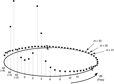
The more conventional way to view a DFT output is to unwrap the spectrum in Figure 3-11 to get the spectrum in Figure 3-12. Figure 3-12 shows some of the additional replications in the spectrum for the 3.4 cycles per sample interval example. Concerning our DFT output asymmetry problem, as some of the input 3.4-cycle signal amplitude leaks into the 2nd bin, the 1st bin, and the 0th bin, leakage continues into the –1st bin, the –2nd bin, the –3rd bin, etc. Remember, the 63rd bin is the –1st bin, the 62nd bin is the –2nd bin, and so on. These bin equivalencies allow us to view the DFT output bins as if they extend into the negative frequency range, as shown in Figure 3-13(a). The result is that the leakage wraps around the m = 0 frequency bin, as well as around the m = N frequency bin. This is not surprising, because the m = 0 frequency is the m = N frequency. The leakage wraparound at the m = 0 frequency accounts for the asymmetry about the DFT's m = 3 bin in Figure 3-8(b).
Figure 3-12. Spectral replication when the DFT input is 3.4 cycles per sample interval.
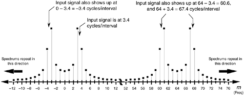
Figure 3-13. DFT output magnitude: (a) when the DFT input is 3.4 cycles per sample interval; (b) when the DFT input is 28.6 cycles per sample interval.
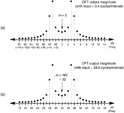
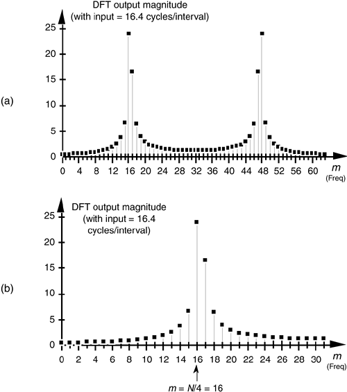
Recall from the DFT symmetry discussion, when a DFT input sequence x(n) is real, the DFT outputs from m = 0 to m = (N/2–1) are redundant with frequency bin values for m > (N/2), where N is the DFT size. The mth DFT output will have the same magnitude as the (N–m)th DFT output. That is, |X(m)| = |X(N–m)|. What this means is that leakage wraparound also occurs about the m = N/2 bin. This can be illustrated using an input of 28.6 cycles per sample interval (32 – 3.4) whose spectrum is shown in Figure 3-13(b). Notice the similarity between Figure 3-13(a) and Figure 3-13(b). So the DFT exhibits leakage wraparound about the m = 0 and m = N/2 bins. Minimum leakage asymmetry will occur near the N/4th bin as shown in Figure 3-14(a) where the full spectrum of a 16.4 cycles per sample interval input is provided. Figure 3-14(b) shows a close-up view of the first 32 bins of the 16.4 cycles per sample interval spectrum.
Figure 3-14. DFT output magnitude when the DFT input is 16.4 cycles per sample interval: (a) full output spectrum view; (b) close-up view showing minimized leakage asymmetry at frequency m = N/4.
You could read about leakage all day. However, the best way to appreciate its effects is to sit down at a computer and use a software program to take DFTs, in the form of fast Fourier transforms (FFTs), of your personally generated test signals like those in Figures 3-7 and 3-8. You can, then, experiment with different combinations of input frequencies and various DFT sizes. You'll be able to demonstrate that DFT leakage effect is troublesome because the bins containing low-level signals are corrupted by the sidelobe levels from neighboring bins containing high-amplitude signals.
Although there's no way to eliminate leakage completely, an important technique known as windowing is the most common remedy to reduce its unpleasant effects. Let's look at a few DFT window examples.
URL http://proquest.safaribooksonline.com/0131089897/ch03lev1sec8
| Amazon | ||
