Section D.1. STATISTICAL MEASURES
D 1 STATISTICAL MEASURES
Consider a continuous sinusoid having a frequency of  o Hz with a peak amplitude of Ap expressed by the equation

Equation (D-1) completely specifies x(t)—that is, we can determine x(t)'s exact value at any given instant. For example, when time t = 1/4 o, we know that x(t)'s amplitude will be Ap and, at the later time t = 1/2fo, x(t)'s amplitude will be zero. On the other hand, we have no definite way to express the successive values of a random function or of random noise.[
 ] There's no equation like Eq. (D-1) available to predict future noise-amplitude values, for example. (That's why they call it random noise.) Statisticians have, however, developed powerful mathematical tools to characterize several properties of random functions. The most important of these properties have been given the names mean, variance, and standard deviation.
[
] We define random noise to be unwanted, unpredictable, disturbances contaminating a signal or a data sequence of interest.
Mathematically, the mean, or average, of N separate values of a sequence x, denoted xave, is defined as [1]
Equation D-2

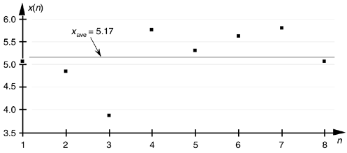
Equation (D-2), already familiar to most people, merely states that the average of a sequence of N numbers is the sum of those numbers divided by N. Graphically, the average can be depicted as that value about which a series of sample values cluster, or congregate, as shown in Figure D-1. If the eight values depicted by the dots in Figure D-1 represent some measured quantity and we applied those values to Eq. (D-2), the average of the series is 5.17, as shown by the dotted line.
Figure D-1. Average of a sequence of eight values.

Now that we've defined average, another key definition is the variance of a sequence, s2, defined as
Equation D-3

Sometimes, in the literature, we'll see s2 defined with a 1/(N–1) factor before the summation instead of the 1/N factor in Eq. (D-3). There are subtle statistical reasons why the 1/(N–1) factor sometimes gives more accurate results [2]. However, when N is greater than, say 20, as it will be for our purposes, the difference between the two factors will have no practical significance.
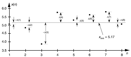
Variance is a very important concept because it's the yardstick with which we measure, for example, the effect of quantization errors and the usefulness of signal-averaging algorithms. It gives us an idea how the aggregate values in a sequence fluctuate about the sequence's average and provides us with a well defined quantitative measure of those fluctuations. (Because the positive square root of the variance, the standard deviation, is typically denoted as s in the literature, we'll use the conventional notation of s2 for the variance.) Equation (D-3) looks a bit perplexing if you haven't seen it before. Its meaning becomes clear if we examine it carefully. The x(1) – xave value in the bracket, for example, is the difference between the x(1) value and the sequence average xave. For any sequence value x(n), the x(n) – xave difference, which we denote as D(n), can be either positive or negative, as shown in Figure D-2. Specifically, the differences D(1), D(2), D(3), and D(8) are negative because their corresponding sequence values are below the sequence average shown by the dotted line. If we replace the x(n) – xave difference terms in Eq. (D-3) with D(n) terms, the variance can be expressed as
Equation D-4

Figure D-2. Difference values D(n) of the sequence in Figure D-1.

The reader might wonder why the squares of the differences are summed, instead of just the differences themselves. If we just add the differences, some of the negative D(n)s will cancel some of the positive D(n)s resulting in a sum that may be too small. For example, if we add the D(n)s in Figure D-2, the positive D(6) and D(7) values and the negative D(3) value will just about cancel each other out and we don't want that. Because we need an unsigned measure of each difference, we use the difference-squared terms as indicated by Eq. (D-4). In that way, individual D(n) difference terms will contribute to the overall variance regardless of whether the difference is positive or negative. Plugging the D(n) values from the example sequence in Figure D-2 into Eq. (D-4), we get a variance value of 0.34. Another useful measure of a signal sequence is the square root of the variance known as the standard deviation. Taking the square root of Eq. (D-3) to get the standard deviation s,
Equation D-5

So far, we have three measurements to use in evaluating a sequence of values: the average xave, the variance s2, and the standard deviation s. Where xave indicates about what constant level the individual sequence values vary, s2 is a measure of the magnitude of the noise fluctuations about the average xave. If the sequence represents a series of random signal samples, we can say that xave specifies the average, or constant, value of the signal. The variance s2 is the magnitude squared, or power, of the fluctuating component of the signal. The standard deviation, then, is an indication of the magnitude of the fluctuating component of the signal.
URL http://proquest.safaribooksonline.com/0131089897/app04lev1sec1
 |
Amazon |  |
