COHERENT AVERAGING | Chapter Eleven. Signal Averaging

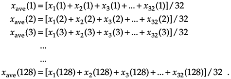
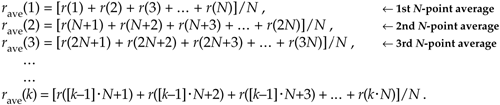
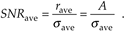
In the coherent averaging process (also known as linear, predetection, or vector averaging), the key feature is the timing used to sample the original signal; that is, we collect multiple sets of signal plus noise samples, and we need the time phase of the signal in each set to be identical. For example, when averaging a sinewave embedded in noise, coherent averaging requires that the phase of the sinewave be the same at the beginning of each measured sample set. When this requirement is met, the sinewave will average to its true sinewave amplitude value. The noise, however, is different in each sample set and will average toward zero.[] The point is that coherent averaging reduces the variance of the noise, while preserving the amplitude of signals that are synchronous, or coherent, with the beginning of the sampling interval. With coherent averaging, we can actually improve the signal-to-noise ratio of a noisy signal. By way of example, consider the sequence of 128 data points plotted in Figure 11-1(a). Those data points represent the time-domain sampling of a single pulse contaminated with random noise. (For illustrative purposes the pulse, whose peak amplitude is 2.5, is shown in the background of Figure 11-1.) It's very difficult to see a pulse in the bold pulse-plus-noise waveform in the foreground of Figure 11-1(a). Let's say we collect 32 sets of 128 pulse-plus-noise samples of the form

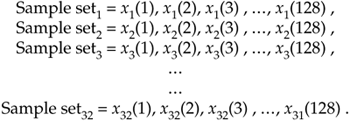
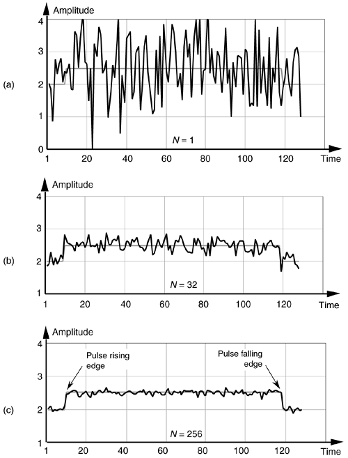
[] Noise samples are assumed to be uncorrelated with each other and uncorrelated with the sample rate. If some component of the noise is correlated with the sample rate, that noise component will be preserved after averaging.

Figure 11-1. Signal pulse plus noise: (a) one sample set; (b) average of 32 sample sets; (c) average of 256 sample sets.

Here's where the coherent part comes in: the signal measurement times must be synchronized, in some manner, with the beginning of the pulse, so that the pulse is in a constant time relationship with the first sample of each sample set. Coherent averaging of the 32 sets of samples, adding up the columns of Eq. (11-4), takes the form of

Equation 11-5

If we perform 32 averages indicated by Eq. (11-5) on a noisy pulse like that in Figure 11-1(a), we'd get the 128-point xave(k) sequence plotted in Figure 11-1(b). Here, we've reduced the noise fluctuations riding on the pulse, and the pulse shape is beginning to become apparent. The coherent average of 256 sets of pulse measurement sequences results in the plot shown in Figure 11-1(c), where the pulse shape is clearly visible now. We've reduced the noise fluctuations while preserving the pulse amplitude. (An important concept to keep in mind is that summation and averaging both reduce noise variance. Summation is merely implementing Eq. (11-5) without dividing the sum by N = 32. If we perform summations and don't divide by N, we merely change the vertical scales for the graphs in Figure 11-1(b) and (c). However, the noise fluctuations will remain unchanged relative to true pulse amplitude on the new scale.)

The mathematics of this averaging process in Eq. (11-5) is both straightforward and important. What we'd like to know is the signal-to-noise improvement gained by coherent averaging as a function of N, the number of sample sets averaged. Let's say that we want to measure some constant time signal with amplitude A, and each time we actually make a measurement we get a slightly different value for A. We realize that our measurements are contaminated with noise such that the nth measurement result r(n) is

Equation 11-6

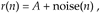
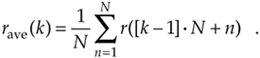
where noise(n) is the noise contribution. Our goal is to determine A when the r(n) sequence of noisy measurements is all we have to work with. For a more accurate estimate of A, we average N separate r(n) measurement samples and calculate a single average value rave. To get a feeling for the accuracy of rave, we decide to take a series of averages rave(k), to see how that series fluctuates with each new average; that is,

Equation 11-7

or, more concisely,

Equation 11-8

To see how averaging reduces our measurement uncertainty, we need to compare the standard deviation of our rave(k) sequence of averages with the standard deviation of the original r(n) sequence.

If the standard deviation of our original series of measurements r(n) is sin, it has been shown [1–5] that the standard deviation of our rave(k) sequence of N-point averages, save, is given by

Equation 11-9

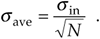
Equation (11-9) is significant because it tells us that the rave(k) series of averages will not fluctuate as much about A as the original r(n) measurement values did; that is, the rave(k) sequence will be less noisy than any r(n) sequence, and the more we average by increasing N, the more closely an individual rave(k) estimate will approach the true value of A.[]

[] Equation (11-9) is based on the assumptions that the average of the original noise is zero and that neither A nor sin change during the time we're performing our averages.

In a different way, we can quantify the noise reduction afforded by averaging. If the quantity A represents the amplitude of a signal and sin represents the standard deviation of the noise riding on that signal amplitude, we can state that the original signal-amplitude-to-noise ratio is

Equation 11-10

Likewise the signal-amplitude-to-noise ratio at the output of an averaging process, SNRave, is defined as

Equation 11-11

Continuing, the signal-to-noise ratio gain, SNRcoh gain, that we've realized through coherent averaging is the ratio of SNRave over SNRin, or

Equation 11-12

Substituting save from Eq. (11-9) in Eq. (11-12), the SNR gain becomes

Equation 11-13

Through averaging, we can realize a signal-to-noise ratio improvement proportional to the square root of the number of signal samples averaged. In terms of signal-to-noise ratio measured in decibels, we have a coherent averaging, or integration, gain of

Equation 11-14

Again, Eqs. (11-13) and (11-14) are valid if A represents the amplitude of a signal and sin represents the original noise standard deviation.

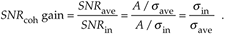
Another way to view the integration gain afforded by coherent averaging is to consider the standard deviation of the input noise, sin, and the probability of measuring a particular value for the Figure 11-1 pulse amplitude. Assume that we made many individual measurements of the pulse amplitude and created a fine-grained histogram of those measured values to get the dashed curve in Figure 11-2. The vertical axis of Figure 11-2 represents the probability of measuring a pulse-amplitude value corresponding to the values on the horizontal axis. If the noise fluctuations follow the well-known normal, or Gaussian distribution, that dashed probability distribution curve is described by

Equation 11-15

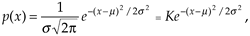
Figure 11-2. Probability density curves of measured pulse amplitudes with no averaging (N = 1) and with N = 32 averaging.

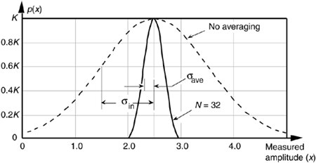
where s = sin and the true pulse amplitude is represented by m = 2.5. We see from that dashed curve that any given measured value will most likely (with highest probability) be near the actual pulse-amplitude value of 2.5. Notice, however, that there's a nonzero probability that the measured value could be as low as 1.0 or as high as 4.0. Let's say that the dashed curve represents the probability curve of the pulse-plus-noise signal in Figure 11-1(a). If we averaged a series of 32 pulse-amplitude values and plotted a probability curve of our averaged pulse-amplitude measurements, we'd get the solid curve in Figure 11-2. This curve characterizes the pulse-plus-noise values in Figure 11-1(b). From this solid curve, we see that there's a very low likelihood (probability) that a measured value, after 32-point averaging, will be less than 2.0 or greater than 3.0.

From Eq. (11-9), we know that the standard deviation of the result of averaging 32 signal sample sets is

Equation 11-16

In Figure 11-2, we can see a statistical view of how an averager's output standard deviation is reduced from the averager's input standard deviation. Taking larger averages by increasing N beyond 32 would squeeze the solid curve in Figure 11-2 even more toward its center value of 2.5, the true pulse amplitude.[]

[] The curves in Figure 11-2 are normalized for convenient illustration. From Eq. (11-15) and assuming that s = 1 when N = 1, then K = 0.3989. When N = 32, the new standard deviation is s' = s/ = 1/ and K = 0.3989 = 2.23.

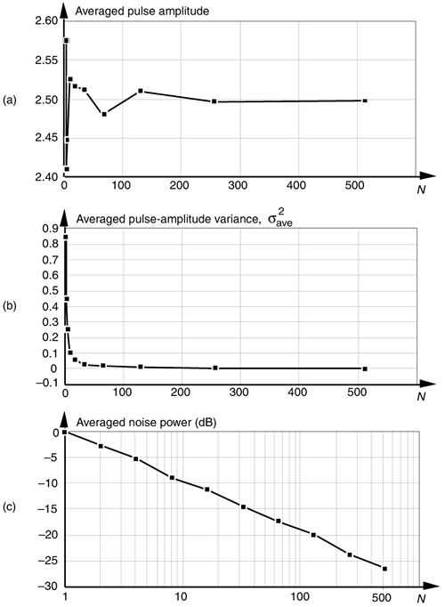
Returning to the noisy pulse signal in Figure 11-1, and performing coherent averaging for various numbers of sample sets N, we see in Figure 11-3(a) that as N increases, the averaged pulse amplitude approaches the true amplitude of 2.5. Figure 11-3(b) shows how rapidly the variance of the noise riding on the pulse falls off as N is increased. An alternate way to see how the noise variance decreases with increasing N is the noise power plotted on a logarithmic scale as in Figure 11-3(c). In this plot, the noise variance is normalized to that noise variance when no averaging is performed, i.e., when N = 1. Notice that the slope of the curve in Figure 11-3(c) closely approximates that predicted by Eqs. (11-13) and (11-14); that is, as N increases by a factor of 10, we reduce the average noise power by 10 dB. Although the test signal in this discussion was a pulse signal, had the signal been sinusoidal, Eqs. (11-13) and (11-14) would still apply.

Figure 11-3. Results of averaging signal pulses plus noise: (a) measured pulse amplitude vs. N; (b) measured variance of pulse amplitude vs. N; (c) measured pulse-amplitude noise power vs. N on a logarithmic scale.