FAST FIR FILTERING USING THE FFT
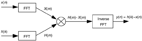
While contemplating the convolution relationships in Eq. (5-31) and Figure 5-41, digital signal processing practitioners realized that convolution could sometimes be performed more efficiently using FFT algorithms than it could be using the direct convolution method. This FFT-based convolution scheme, called fast convolution, is diagrammed in Figure 13-28.
Figure 13-28. Processing diagram of fast convolution.
The standard convolution equation for an M-tap nonrecursive FIR filter, given in Eq. (5-6) and repeated here, is
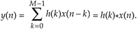
where h(k) is the impulse response sequence (coefficients) of the FIR filter and the * symbol indicates convolution. It has been shown that when the final y(n) output sequence has a length greater than 30, the process in Figure 13-28 requires fewer multiplications than implementing the convolution expression in Eq. (13-67) directly. Consequently, this fast convolution technique is a very powerful signal processing tool, particularly when used for digital filtering. Very efficient FIR filters can be designed using this technique because, if their impulse response h(k) is constant, then we don't have to bother recalculating H(m) each time a new x(n) sequence is filtered. In this case the H(m) sequence can be precalculated and stored in memory.
The necessary forward and inverse FFT sizes must of course be equal, and are dependent upon the length of the original h(k) and x(n) sequences. Recall from Eq. (5-29) that if h(k) is of length P and x(n) is of length Q, the length of the final y(n) sequence will be (P+Q–1). For this fast convolution technique to give valid results, the forward and inverse FFT sizes must be equal and greater than (P+Q–1). This means that h(k) and x(n) must both be padded with zero-valued samples, at the end of their respective sequences, to make their lengths identical and greater than (P+Q–1). This zero padding will not invalidate the fast convolution results. So to use fast convolution, we must choose an N-point FFT size such that N  (P+Q–1) and zero pad h(k) and x(n) so they have new lengths equal to N.
An interesting aspect of fast convolution, from a hardware standpoint, is that the FFT indexing bit-reversal problem discussed in Sections 4.5 and 4.6 is not an issue here. If the identical FFT structures used in Figure 13-28 result in X(m) and H(m) having bit-reversed indices, the multiplication can still be performed directly on the scrambled H(m) and X(m) sequences. Then an appropriate inverse FFT structure can be used that expects bit-reversed input data. That inverse FFT then provides an output y(n) whose data index is in the correct order!
URL http://proquest.safaribooksonline.com/0131089897/ch13lev1sec10
| Amazon | ||
