GENERATING NORMALLY DISTRIBUTED RANDOM DATA | Chapter Thirteen. Digital Signal Processing Tricks

Section D.4 in Appendix D discusses the normal distribution curve as it relates to random data. A problem we may encounter is how actually to generate random data samples whose distribution follows that normal (Gaussian) curve. There's a straightforward way to solve this problem using any software package that can generate uniformly distributed random data, as most of them do[27]. Figure 13-29 shows our situation pictorially where we require random data that's distributed normally with a mean (average) of m' and a standard deviation of s', as in Figure 13-29(a), and all we have available is a software routine that generates random data that's uniformly distributed between zero and one as in Figure 13-29(b).

Figure 13-29. Probability distribution functions: (a) Normal distribution with mean = m', and standard deviation s'; (b) Uniform distribution between zero and one.

As it turns out, there's a principle in advanced probability theory, known as the Central Limit Theorem, that says when random data from an arbitrary distribution is summed over M samples, the probability distribution of the sum begins to approach a normal distribution as M increases[28–30]. In other words, if we generate a set of N random samples that are uniformly distributed between zero and one, we can begin adding other sets of N samples to the first set. As we continue summing additional sets, the distribution of the N-element set of sums becomes more and more normal. We can sound impressive and state that "the sum becomes asymptotically normal." Experience has shown that for practical purposes, if we sum M 30 times, the summed data distribution is essentially normal. With this rule in mind, we're half way to solving our problem.

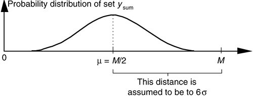
After summing M sets of uniformly distributed samples, the summed set ysum will have a distribution as shown in Figure 13-30.

Figure 13-30. Probability distribution of the summed set of random data derived from uniformly distributed data.

Because we've summed M sets, the mean of ysum is m = M/2. To determine ysum's standard deviation s, we assume that the six sigma point is equal to M–m. That is,

That assumption is valid because we know that the probability of an element in ysum being greater that M is zero, and the probability of having a normal data sample at six sigma is one chance in six billion, or essentially zero. Because m = M/2, from Eq. (13-68), ysum's standard deviation is set to

Equation 13-69

To convert the ysum data set to our desired data set having a mean of m' and a standard deviation of s', we :

subtract M/2 from each element of ysum to shift its mean to zero,
ensure that 6s' is equal to M/2 by multiplying each element in the shifted data set by 12s'/M, and
center the new data set about the desired m' by adding m' to each element of the new data.

If we call our desired normally distributed random data set ydesired, then the nth element of that set is described mathematically as

Equation 13-70

Our discussion thus far has had a decidedly software algorithm flavor, but hardware designers also occasionally need to generate normally distributed random data at high speeds in their designs. For you hardware designers, Reference [30] presents an efficient hardware design technique to generate normally distributed random data using fixed-point arithmetic integrated circuits.

The above method for generating normally distributed random numbers works reasonably well, but its results are not perfect because the tails of the probability distribution curve in Figure 13-30 are not perfectly Gaussian.[] An advanced, and more statistically correct (improved randomness), technique that you may want to explore is called the Ziggurat method[31–33].