Some Definitions

What Is an Image?

Naturally, we are only interested in a definition of "image" that is essential for image processing. A common method is to define an image I as a rectangular matrix (called image matrix)

Equation 1.1

with image rows (defining the row counter or row index x ) and image columns (column counter or column index y ). One row value together with a column value defines a small image area called pixel (from picture element), which is assigned a value representing the brightness of the pixel.

One possibility is to assign gray-scale values s ( x,y ) of the gray-scale set G = {0,1,...,255}. The gray-scale value 0 corresponds to black and 255 to white. Such an image is called an 8-bit gray-scale image with

Equation 1.2

Exercise 1.1: Image Creation.

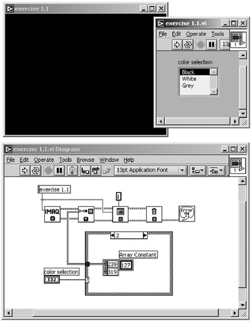
Create the LabVIEW program shown in Figure 1.4. It shows that a simple image can be created by a rectangular matrix. The IMAQ function ArrayToImage provides the conversion from data type "array" to data type "image." Now you can assign the matrix elements (identical) values between 0 and 255.

Moreover, Figure 1.4 shows the general handling of the data type "image" in LabVIEW and IMAQ Vision. The first step is to reserve a memory area with the function IMAQ Create ; when the program stops, the memory area should be released again with IMAQ Dispose . The image itself is visible only if you show it on the screen with the function IMAQ WindDraw . Note that IMAQ Vision uses additional windows for images; the front panel window of LabVIEW does not offer any controls or indicators.

The image size used in this exercise is 320 x 240 pixels, that is, a quarter of VGA resolution of 640 x 480 pixels, and is common with video cameras . Note that the matrix indices in LabVIEW start with 0; the maximum row and column indices therefore have the values 319 and 239.

 

Figure 1.4. Definition of an Image as a Rectangular Matrix

The assignment to the 8-bit gray-scale set G is arbitrary. Sometimes an image pixel is represented by less than the 256 gray-scale values; a binary image consists only of the values 0 and 1 (black and white). Therefore, 1 bit per pixel can be sufficient for image description.

On the other hand, sometimes 256 values may not be enough for displaying all of the information an image contains. Typically, a color image cannot be represented by the model shown in Eq. (1.1). In that case, we can extend the image I by using more planes and then we talk about multiplane images :

Equation 1.3

 

with n as the plane counter . Figure 1.5 shows a three-plane image used for storing color information; the color red is assigned to plane 0, green to plane 1, and blue to plane 2. A single pixel of an N -plane image is represented by an N -dimensional vector

Figure 1.5. Definition of a Color Image as Multiplane Image

Equation 1.4

 

where the components g n are elements of the gray-scale set G [12].

Note that Figure 1.5 also shows position and orientation of the row and column indices. The starting point for both is the upper-left corner of the image; the row index x increases to the bottom, the column index y to the right.

Exercise 1.2: Color Image.

Create the LabVIEW program shown in Figure 1.6. Read in any desired color image through the dialog box; it is important that the image be defined as an RGB image by the function IMAQ Create ; otherwise , the planes cannot be extracted.

Select the desired image plane with the control element "color plane," watch the display information, and compare it with the real colors of the image. You can try the planes Hue, Saturation, Luminance, Value, and Intensity as well; they are related to other color models, which are discussed later in this book and may give better results in color recognition tasks .

 

Figure 1.6. Definition of an RGB-Color Image

The Difference: Image Processing or Image Analysis?

We have already heard these terms several times in this book. Usually, it can be assumed that both expressions have about the same meaning, but if we go deeper into detail, some differences can be found.

First of all, please notice that the following definitions are subjective ; they are mine, and they differ a little bit from those of National Instruments. Nevertheless, I believe they make sense.

I use the term image processing for all manipulations on an image (as defined above) if the output of the manipulation is again an image. For example, take a look at Figure 1.7. It shows two images; the right one is the result of manipulation of the left one. It is easy to see (and we will also learn later) that this manipulation influences the brightness and the contrast of the original image. Obviously, the output is an image.

Figure 1.7. Image Processing Example. The right image results from brightness and contrast manipulation of the left one.

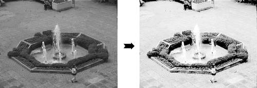
Image analysis is used when the output of a manipulation is not an image. Let us look at the example in Figure 1.8. We can see some kind of an image in the right as well, but the result of the manipulation is a number: 5; this means that five objects were detected in the left image.

Figure 1.8. Image Analysis Example. The object detection algorithm returns the number of detected objects in the left image.

The images were taken from an application we discuss in Chapter 5: Object Detection and Counting in Public Places .

Finally: Machine Vision

The term Machine Vision or Computer Vision is often used for the entire subject, including image processing and image analysis. If we really want to define Machine Vision, we have to first clarify what vision itself is.

Undoubtedly, vision is the human sense that provides most of the information a human has to process. Rough estimations say that the data rate for continuous viewing is about 10 megabits per second. It is obvious that this huge amount of data cannot be processed in real time (defined in the next section); it has to be filtered by the visual cortex .

We define Machine Vision as high-level applications that come close to human vision capabilities (remember the car example); but we should always keep in mind that these human capabilities for recognition will not be reached by Machine Vision; for reliability, speed and accuracy on the other hand, they will.

Real Time or "Really Fast"?

Mostly, it is assumed that a system running under real-time conditions should react "really fast," thus providing reaction times that are as short as possible. It is assumed that a very fast PC using Windows as the operating system is capable of providing real-time conditions.

This assumption is definitely incorrect. Real time simply means that every operation has to be completed within acceptable delay times, however the system ensures completion. Therefore, Windows as a quite "unreliable" operating system is not suitable for most real-time applications. [3]

[3] On the other hand, that does not mean that Windows is "real-time unsuitable" in general.

Virtual Instrumentation

According to a course manual from National Instruments, one of the " creators " of virtual instrumentation , this term is defined as

• the use of industry-standard computers,
• equipped with user -friendly application software,
• cost-effective hardware and driver software

that together perform the functions of traditional instruments. The advantages of virtual instrumentation are obvious:

• Virtual instruments are easily adaptable to changing demands;
• the user interface can be adapted to the needs of different users;
• user interface, hardware, and application software are suitable for modular use.

Introduction to IMAQ Vision Builder