Pixel Value Analysis

Although this chapter would be the correct place for the histogram function, we already discussed it in Chapter 4 on page 151, so go there for detailed information. Another function, which gives a pixel value distribution, is discussed here: the line profile .

Line Profile

The line profile function simply visualizes the pixel values (gray-level values for gray-scaled images) along a line, which must be specified by its coordinates or results from a manually drawn line. Figure 5.1 shows this function in the IMAQ Vision Builder.

Figure 5.1. Line Profile Function in IMAQ Vision Builder

Directly in LabVIEW and IMAQ Vision, you must specify the line coordinates by using an array control or an array constant. Exercise 5.1 shows how.

Exercise 5.1: Line Profile in Images.

Create a LabVIEW VI that draws the pixel value profile along a previously defined line in an image, using the function IMAQ Line Profile (found in Motion and Vision / Image Processing / Analysis). Figures 5.2 and 5.3 show a possible solution.

 

Actually, it is more convenient to draw the line directly in the image, using a function like IMAQ SelectLine , much like the behavior of IMAQ Vision Builder. I leave the extension of Exercise 5.1 up to you.

Figures 5.2 and 5.3 also show another interesting group of VIs: the overlay functions. You can find them in Motion and Vision / Vision Utilities / Overlay (see Figure 5.4); they are useful if you want to provide additional information in the IMAQ image window itself.

Figure 5.2. Line Profile of an Image

Figure 5.3. Diagram of Exercise 5.1

Figure 5.4. Menu Palette Containing Overlay Functions

Almost all overlay functions have the following inputs:

• the original image;
• the item type, which should be placed over the original image, for example:
  • single points,
  • lines (single or multiple),
  • rectangles,
  • circles and ovals,
  • text,
  • bitmaps;
• at least one coordinate pair, specifying where to place the overlay;
• the color of the overlay (not with bitmaps).

The only output is the resulting image with the overlay information, so the overlay is typically placed between processing or analysis functions and the IMAQ WindDraw function.

I used two different overlay functions in Exercise 5.1. As you can see in Figure 5.3, the first one simply draws the line you can specify in the Line Coordinates control. Note that the line coordinates are stored in a 4 x 1 array; but the data required by IMAQ OverlayLine is two clusters of the coordinates of the start and the end point, respectively.

The second function is more complex; the exercise uses the gray-scale values of the line profile, recalculates them so that they can be displayed in the IMAQ window, and displays them on top of the red line. Red is the default color of the overlay structure; the profile color can be changed by use of a color constant, for example, to yellow.

Quantify Areas

The quantify function can be used to obtain simple statistical data about the gray-level values of pixels in a specified region. We try this exercise in IMAQ Vision Builder, when you select the menu item Quantify in the Grayscale menu. After selecting a region of interest, you can view the results (Figure 5.5).

Figure 5.5. Quantifying Image Areas with IMAQ Vision Builder

The values provided by IMAQ Vision Builder using the quantify function are:

• mean value;
• standard variation;
• minimum value, and
• maximum value.

You will get an interesting result if you let IMAQ Vision Builder construct a LabVIEW VI (Figure 5.6). Obviously, the Vision Builder does not use the function IMAQ Quantify , as we expected; it uses a function IVB Quantify instead. IMAQ Vision Builder uses the IVB functions for the automated construction of VIs because they provide a more standardized system for input and output variables .

Figure 5.6. LabVIEW Quantify VI Generated with IMAQ Vision Builder

Figure 5.7. IVB (IMAQ Vision Builder) Functions

Figure 5.7 shows the difference between the two functions used in this exercise. You can find more IVB functions following the directory path (depending on your system) ...National InstrumentsIMAQ Vision Builder 6programextaddons .

Centroid Function

The function IMAQ Centroid calculates the Center of Energy of either a specified region or the entire image. You can watch the results by selecting the Centroid function in IMAQ Vision Builder and by specifying various areas with different brightness distributions (Figure 5.8).

Figure 5.8. Centroid Function (Center of Energy)

Linear Averages

We use overlay functions in the next exercise, with the IMAQ Vision function IMAQ LinearAverage . The function itself is simple; it calculates the mean line profiles in x and in y direction, respectively.

Exercie 5.2: Linear Averages.

Calculate the mean linear averages in x and in y direction, using the function IMAQ LinearAverage . Display the line profiles in both directions directly in the image, similarly to the solution in Exercise 5.1. Compare your solution to Figures 5.9 and 5.10.

 

Figure 5.9. Linear Average of Pixel Values in x and y Direction

Figure 5.10. Diagram of Exercise 5.2

The function IMAQ LinearAverage also enables you to specify only a region of the image, in which you want the average line profiles to be calculated. To do this, you add an array constant or an array control and enter the coordinates of an Optional Rectangle.

Edge Detection

In Edge Detection and Enhancement in Chapter 4, we discussed only edge enhancing, because we did not get any information (in numbers [1] ) about the location of the edge. We can get numerical information in the following exercises.

[1] Remember the definitions of image processing and image analysis and the resulting difference between them.

Simple Edge Detector

We can use the information returned by the line profile function to determine edges along the line by simply checking whether the gray-level value of the pixels exceeds a previously given threshold value, as in Exercise 5.3.

Exercise 5.3: Simple Edge Detector.

Create a LabVIEW VI that uses the line profile information for the realization of a simple edge detector, using the functions IMAQ Line Profile and IMAQ SimpleEdge (can be found in Motion and Vision / Machine Vision / Caliper). See a possible solution in Figures 5.11 and 5.12.

 

Figure 5.11. Simple Edge Detector

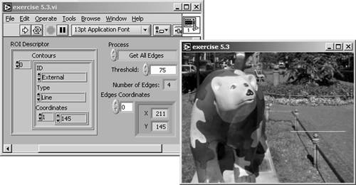
Figure 5.12. Diagram of Exercise 5.3

Again, we use an overlay function to visualize the line on which the edges should be detected . You can extend Exercise 5.3 by indicating the edges, for example, by drawing small circles at the edge location, using IMAQ OverlayOval . The application example Feedback Form Reader on page 304 offers a possible solution.

Exercise 5.3 also uses the function IMAQ ROIProfile , which converts a region of interest (ROI) to pixel coordinates. An ROI limits the desired operation to a smaller area of the image. IMAQ Vision provides a number of ROI functions in Motion and Vision / Vision Utilities / Region of Interest (see Figure 5.13).

Figure 5.13. Menu Palette Containing ROI Functions

An ROI is decsribed by the ROI descriptor, which is a cluster containing the following:

• a bounding rectangle , and
• a regions list , an array of clusters containing
• a contour identifier (0 for exterior and 1 for interior contour),
• the contour type , for example, rectangle or oval,
• a list of points describing the contour.

You can read more about ROIs in [5].

IMAQ Edge Detection Tool

If the function IMAQ SimpleEdge does not meet your needs, you can use the function IMAQ EdgeTool (to be found in Motion and Vision / Machine Vision / Caliper). Here, you can specify additional parameters like the slope steepness or subpixel accuracy.

Exercise 5.4: Complex Edge Tool.

It is easy to change Exercise 5.3 by replacing IMAQ SimpleEdge with IMAQ EdgeTool and to modify the necessary controls. You will need numeric controls for Contrast, Filter Width, and slope Steepness. I did not wire the input for subpixel information, which may enable higher resolution than the pixel size and uses special interpolation functions. Try it yourself, starting with Figures 5.14 and 5.15.

 

Figure 5.14. Edge Detection Tool

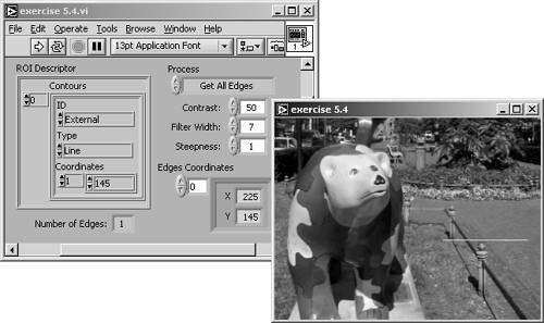
Figure 5.15. Diagram of Exercise 5.4

Peak-Valley Detection

The next function is not really an edge detector; it detects peaks or valleys of a line profile. In addition, it returns information about the peaks or valleys, including the second derivatives.

Exercise 5.5: Peak-Valley Detector.

In this exercise, use the IMAQ Vision function IMAQ Peak-Valley Detector . Display the line in the original image as in the exercises before and the gray-level profile in a waveform graph. Overlay this graph with the detected peaks or valleys.

I used a trick for the overlay information: the XY graph in the diagram (Figure 5.17) is a transparent one and placed over the waveform graph. Because the waveform graph has autoscaled x and y axes, the ranges of both axes are transferred to the XY graph by Property Nodes. You have to turn the autoscale mode off in the XY graph. See also Figure 5.16.

 

Figure 5.16. Detecting Peaks and Valleys of a Line Profile

Figure 5.17. Diagram of Exercise 5.5

Another group of VIs, which can be found in Motion and Vision / Vision Utilities / Pixel Manipulation, is used in Exercise 5.5. We have to use the function IMAQ GetPixelLine here because the peak-valley detector needs an array containing the line profile information as input. The other functions, shown in Figure 5.18, can be used to either set or get the pixel values of image rows, columns , or lines, specified by their coordinates.

Figure 5.18. Menu Palette Containing Pixel Manipulation Functions

Locating Edges

In our next exercise we try to build an almost complete machine vision application, using the function IMAQ Find Horizontal Edge (found in Motion and Vision / Machine Vision / Locate Edges). The VI should locate horizontal edges of objects in a specified ROI of the image.

Exercise 5.6: Finding Horizontal Edges.

You can see that the diagram of this exercise (Figure 5.19) is small and simple, although the application itself is very powerful. The reason is that the function IMAQ Find Horizontal Edge already contains a full machine vision application. All you need to do is wire a cluster for the settings, including filter settings (similar to Exercise 5.4), the scan direction (left to right, right to left, top to bottom, or bottom to top), and check boxes for the overlay of information to the original image. Another cluster control specifies the search region within the image.

 

Figure 5.19. Locating Edges in Images

This exercise VI also specifies the edge coordinates inside the ROI. Because we are looking for straight edges here, the coordinates are used to calculate a line that fits the edge of the object. In Figure 5.19 I used our bear image, but it is obvious that this image is not appropriate for this function.

Figure 5.20 shows the application of Exercise 5.6 to an image showing the top view of a small motor, which is common in household appliances and toys. The image is prepared for image vision by maximizing the contrast ratio; it is almost binary. If you want to use your own images, you can modify contrast, brightness, and saturation with a program like Corel Photo Paint; of course, you can also use IMAQ Vision to do this.

Figure 5.20. Locating Horizontal Edges

Let's now extend Exercise 5.6 so that circular edges can be detected.

Exercise 5.7: Finding Circular Edges.

Modify Exercise 5.6 by adding the function IMAQ Find Circular Edge . Use both edge location functions to detect horizontal and circular edges in the motor image by adjusting the parameters of the Rectangle and the Circle or Annulus cluster control. The Settings controls are used for both functions; only the Scan Direction control is different. See Figure 5.21 for the front panel, Figure 5.22 for the diagram, and Figure 5.23 for a result.

 

Figure 5.21. Locating Horizontal and Circular Edges

Figure 5.22. Diagram of Exercise 5.7

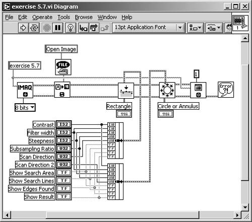
Figure 5.23. Edge-Locating Result (Motor)

Other functions in the submenu Motion and Vision / Machine Vision / Locate Edges provide the location of vertical edges ( IMAQ Find Vertical Edge ) and circular edges ( IMAQ Find Concentric Edge ). You should have no problem now in building your own edge-locating applications.

Morphology Analysis

We now return to the binary morphology VIs of Chapter 4. Some of them, like skeleton or skiz functions, were already close to analysis functions according to our definition.

Distance and Danielsson

The IMAQ Distance and the IMAQ Danielsson functions, for example, provide information about the distance of an object (white areas) from the background border (black areas) and display this information by using colors of the binary palette.

Exercise 5.8: Distance and Danielsson.

Take an exercise from Chapter 4, for example, Exercise 4.20, and insert the function IMAQ Distance . You may provide the function IMAQ Danielsson as well and put it in a Case Structure, which can be used to select the function type. See Figure 5.24 for the front panel and Figure 5.25 for the diagram.

 

Figure 5.24. Distance Indication in Binary Images

Figure 5.25. Diagram of Exercise 5.8

Figure 5.24 shows the result of the distance function in the binary bear image. Again, it is clear that this image is not appropriate for this function, although the principle is clear: Each object shows a number of color lines, which indicate the distance to the background.

Figure 5.26 shows the same function applied to the motor image of the last exercise. The effect of the distance function gets even clearer, but look at the areas near the straight edges of the image. Inside these four regions, which look like a big "V," are pixels with the same distance mapping. But it can be clearly seen that their distance to the next black pixel is different ; this algorithm is obviously not very accurate.

Figure 5.26. Distance Function Applied to a Binary Motor Image

The Danielsson function is based on an algorithm called Euclidean Distance Mapping and was introduced by P. E. Danielsson in 1980. [2] As Figure 5.27 shows, the algorithm shows more reliable results.

[2] P. E. Danielsson: "Euclidean Distance Mapping." Computer Graphics and Image Processing , Volume 14, 1980, pp. 227-248.

Danielsson himself calls the algorithms he developed "Four-point Sequential Euclidean Distance Mapping" (4SED) and "Eight-point Sequential Euclidean Distance Mapping" (8SED), respectively, which reminds us of Figure 4.48, showing the definition of connectivity =4 and connectivity =8.

Figure 5.27. Danielsson Function Applied to a Binary Motor Image

Labeling and Segmentation

We also discussed functions like IMAQ Convex , which require "labeling" of objects in a binary image, which means that these objects are classified and numbered. The next exercise creates a labeled binary image.

Exercise 5.9: Labeling Particles.

Modify Exercise 5.8 by inserting the function IMAQ Label (to be found in Motion and Vision / Image Processing / Processing). Figure 5.28 shows that the labeling is visualized by assignment of a color of the binary palette (visible by different gray levels in Figure 5.28). Use a numeric indicator to display the number of objects. See Figure 5.29 for the diagram.

 

Figure 5.28. Labeling of Binary Images

Figure 5.29. Diagram of Exercise 5.9

The function IMAQ Segmentation requires a labeled binary image and expands the objects until each object reaches its neighbors. The expanding is done by multiple dilation functions until the image contains no more background areas.

Exercise 5.10: Segmentation of Images.

Insert the function IMAQ Segmentation in Exercise 5.9, so that it follows IMAQ Label . It is useful to display the labeled image as well as the segmented image, so you have to do some changes in the wiring. See Figure 5.30 for the panel and the results and Figure 5.31 for the diagram.

 

Figure 5.30. Segmentation of Labeled Binary Images

Figure 5.31. Diagram of Exercise 5.10

The segmentation of a binary image can be interpreted as the calculation of an influence region of each labeled object. Figure 5.32 shows the labeling and segmentation result for the motor image.

Figure 5.32. Segmentation Result of the Motor Image

Circle Detection

The next function, IMAQ Find Circles , detects circles in binary images and is therefore very similar to the function IMAQ Find Circular Edge . The only difference is that IMAQ Find Circles searches not only for edges, but for the entire circle area. We test this function in the next exercise.

Exercise 5.11: Finding Circles.

Modify Exercise 5.9 ( not 5.10) by replacing IMAQ Label with IMAQ Find Circles . Provide numeric controls for the specification of the minimum and the maximum circle radius value, and indicators for the number of detected circles and the circles data. See Figure 5.33 for the panel, Figure 5.34 for results, and Figure 5.35 for the diagram.

 

Figure 5.33. Circle Detection Exercise

Circles Data is an array of clusters, one cluster for each detected circle, consisting of the following elements:

• the x coordinate,
• the y coordinate,
• the radius of the detected circle, and
• the entire circle area.

We need a new binary image for the testing of this function; you can either use dc_motor_bin3.png from the attached CD or modify dc_motor.png , for example, by using IMAQ Vision Builder, by performing the following steps:

1. Load dc_motor.png in the IMAQ Vision Builder.
2. Apply a threshold operation with a minimum value of 30 and a maximum of 190.
3. Invert the image.
4. Remove small objects from the Adv. Morphology menu (two iterations).
5. Invert the image.
6. Remove small objects (seven iterations, hexagonal connectivity).
7. Invert the image.

Figure 5.34 shows the result if the generated binary motor image is processed ; four circles should be detected. If you need more information about the generation of the image we use, here is the entire IMAQ Vision Builder script.

Figure 5.34. Circle Detection Result of the Modified Motor Image

Figure 5.35. Diagram of Exercise 5.11

IMAQ Vision Builder 6.0
List of functions generated :
Sunday, 08. September 2002 18:54

STEP #1 Threshold : Manual Threshold
IMAQ Vision VI IMAQ Threshold
C Function imaqThreshold
Visual Basic Methods CWIMAQVision.Threshold
Parameters:
Range.Lower value Float (SGL) 30,118111
Range.Upper value Float (SGL) 189,744095

IMAQ Vision VI IMAQ Cast Image
C Function imaqCast
Visual Basic Methods CWIMAQVision.Cast
Parameters:
Image Type Long (I32) 0

Connections:
Connect output "Image Dst Out" of "IMAQ Threshold"
to input "Image Src" of "IMAQ Cast Image".
Connect output "error out" of "IMAQ Threshold" to
input "error in (no error)" of "IMAQ Cast Image".

STEP #2 Invert Binary Image
IMAQ Vision VI IVB Binary Inverse.vi
C Function imaqLookup
Visual Basic Methods CWIMAQVision.UserLookup
Parameters:

STEP #3 Adv. Morphology : Remove small objects
IMAQ Vision VI IMAQ RemoveParticle
C Function imaqSizeFilter
Visual Basic Methods CWIMAQVision.RemoveParticle
Parameters:
Connectivity 4/8 Boolean FALSE
Square / Hexa Boolean FALSE
Nb of Iteration Long (I32) 2
Low Pass / High Pass Boolean FALSE

STEP #4 Invert Binary Image
IMAQ Vision VI IVB Binary Inverse.vi
C Function imaqLookup
Visual Basic Methods CWIMAQVision.UserLookup
Parameters:

STEP #5 Adv. Morphology : Remove small objects
IMAQ Vision VI IMAQ RemoveParticle
C Function imaqSizeFilter
Visual Basic Methods CWIMAQVision.RemoveParticle
Parameters:
Connectivity 4/8 Boolean FALSE
Square / Hexa Boolean TRUE
Nb of Iteration Long (I32) 7
Low Pass / High Pass Boolean FALSE

STEP #6 Invert Binary Image
IMAQ Vision VI IVB Binary Inverse.vi
C Function imaqLookup
Visual Basic Methods CWIMAQVision.UserLookup
Parameters:

Comment: Display your image with a Binary palette.

Quantitative Analysis