AN INTRODUCTION TO FINITE IMPULSE RESPONSE (FIR) FILTERS
First of all, FIR digital filters use only current and past input samples, and none of the filter's previous output samples, to obtain a current output sample value. (That's also why FIR filters are sometimes called nonrecursive filters.) Given a finite duration of nonzero input values, the effect is that an FIR filter will always have a finite duration of nonzero output values, and that's how FIR filters got their name. So, if the FIR filter's input suddenly becomes a sequence of all zeros, the filter's output will eventually be all zeros. While not sounding all that unusual, this characteristic is however, very important, and we'll soon find out why, as we learn more about digital filters.
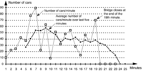
FIR filters use addition to calculate their outputs in a manner much the same as the process of averaging uses addition. In fact, averaging is a kind of FIR filter that we can illustrate with an example. Let's say we're counting the number of cars that pass over a bridge every minute, and we need to know the average number of cars per minute over five-minute intervals; that is, every minute we'll calculate the average number of cars/minute over the last five minutes. If the results of our car counting for the first ten minutes are those values shown in the center column of Table 5-1, then the average number of cars/minute over the previous five one-minute intervals is listed in the right column of the table. We've added the number of cars for the first five one-minute intervals and divided by five to get our first five-minute average output value, (10+22+24+42+37)/5 = 27. Next we've averaged the number of cars/minute for the second to the sixth one-minute intervals to get our second five-minute average output of 40.4. Continuing, we average the number of cars/minute for the third to the seventh one-minute intervals to get our third average output of 53.8, and so on. With the number of cars/minute for the one-minute intervals represented by the dashed line in Figure 5-2, we show our five-minute average output as the solid line. (Figure 5-2 shows cars/minute input values beyond the first ten minutes listed in Table 5-1 to illustrate a couple of important ideas to be discussed shortly.)
Figure 5-2. Averaging the number of cars/minute. The dashed line shows the individual cars/minute, and the solid line is the number of cars/minute averaged over the last five minutes.

Table 5-1. Values for the Averaging Example
|
Minute index |
Number of cars/minute over the last minute |
Number of cars/minute averaged over the last five minutes |
|---|---|---|
|
1 |
10 |
– |
|
2 |
22 |
– |
|
3 |
24 |
– |
|
4 |
42 |
– |
|
5 |
37 |
27 |
|
6 |
77 |
40.4 |
|
7 |
89 |
53.8 |
|
8 |
22 |
53.4 |
|
9 |
63 |
57.6 |
|
10 |
9 |
52 |
There's much to learn from this simple averaging example. In Figure 5-2, notice that the sudden changes in our input sequence of cars/minute are flattened out by our averager. The averager output sequence is considerably smoother than the input sequence. Knowing that sudden transitions in a time sequence represent high frequency components, we can say that our averager is behaving like a low-pass filter and smoothing sudden changes in the input. Is our averager an FIR filter? It sure is—no previous averager output value is used to determine a current output value; only input values are used to calculate output values. In addition, we see that, if the bridge were suddenly closed at the end of the 19th minute, the dashed line immediately goes to zero cars/minute at the end of the 20th minute, and the averager's output in Figure 5-2 approaches and settles to a value of zero by the end of the 24th minute.
Figure 5-2 shows the first averager output sample occurring at the end of the 5th minute because that's when we first have five input samples to calculate a valid average. The 5th output of our averager can be denoted as yave(5) where

In the general case, if the kth input sample is x(k), then the nth output is
Equation 5-2

Look at Eq. (5-2) carefully now. It states that the nth output is the average of the nth input sample and the four previous input samples.
We can formalize the digital filter nature of our averager by creating the block diagram in Figure 5-3 showing how the averager calculates its output samples.
Figure 5-3. Averaging filter block diagram when the fifth input sample value, 37, is applied.

This block diagram, referred to as the filter structure, is a physical depiction of how we might calculate our averaging filter outputs with the input sequence of values shifted, in order, from left to right along the top of the filter as new output calculations are performed. This structure, implementing Eqs. (5-1) and (5-2), shows those values used when the first five input sample values are available. The delay elements in Figure 5-3, called unit delays, merely indicate a shift register arrangement where input sample values are temporarily stored during an output calculation.
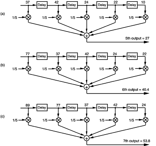
In averaging, we add five numbers and divide the sum by five to get our answer. In a conventional FIR filter implementation, we can just as well multiply each of the five input samples by the coefficient 1/5 and then perform the summation as shown in Figure 5-4(a). Of course, the two methods in Figures 5-3 and 5-4(a) are equivalent because Eq. (5-2) describing the structure shown in Figure 5-3 is equivalent to
Equation 5-3

Figure 5-4. Alternate averaging filter structure: (a) input values used for the 5th output value; (b) input values used for the 6th output value; (c) input values used for the 7th output value.

that describes the structure in Figure 5-4(a).[ ]
]
[
] We've used the venerable distributive law for multiplication and addition of scalars, a(b+c+d) = ab+ac+ad, in moving Eq. (5-2)'s factor of 1/5 inside the summation in Eq. (5-3).
Let's make sure we understand what's happening in Figure 5-4(a). Each of the first five input values are multiplied by 1/5, and the five products are summed to give the 5th filter output value. The left to right sample shifting is illustrated in Figures 5-4(b) and 5-4(c). To calculate the filter's 6th output value, the input sequence is right shifted discarding the 1st input value of 10, and the 6th input value 77 is accepted on the left. Likewise, to calculate the filter's 7th output value, the input sequence is right shifted discarding the 2nd value of 22, and the 7th input value 89 arrives on the left. So, when a new input sample value is applied, the filter discards the oldest sample value, multiplies the samples by the coefficients of 1/5, and sums the products to get a single new output value. The filter's structure using this bucket brigade shifting process is often called a transversal filter due to the cross-directional flow of the input samples. Because we tap off five separate input sample values to calculate an output value, the structure in Figure 5-4 is called a 5-tap FIR filter, in digital filter vernacular.
One important and, perhaps, most interesting aspect of understanding FIR filters is learning how to predict their behavior when sinusoidal samples of various frequencies are applied to the input, i.e., how to estimate their frequency-domain response. Two factors affect an FIR filter's frequency response: the number of taps and the specific values used for the multiplication coefficients. We'll explore these two factors using our averaging example and, then, see how we can use them to design FIR filters. This brings us to the point where we have to introduce the C word: convolution. (Actually, we already slipped a convolution equation in on the reader without saying so. It was Eq. (5-3), and we'll examine it in more detail later.)
URL http://proquest.safaribooksonline.com/0131089897/ch05lev1sec1
 |
Amazon |  |
