SAMPLING BANDPASS SIGNALS
Although satisfying the majority of sampling requirements, the sampling of low-pass signals, as in Figure 2-6, is not the only sampling scheme used in practice. We can use a technique known as bandpass sampling to sample a continuous bandpass signal that is centered about some frequency other than zero Hz. When a continuous input signal's bandwidth and center frequency permit us to do so, bandpass sampling not only reduces the speed requirement of A/D converters below that necessary with traditional low-pass sampling; it also reduces the amount of digital memory necessary to capture a given time interval of a continuous signal.
By way of example, consider sampling the band-limited signal shown in Figure 2-7(a) centered at fc = 20 MHz, with a bandwidth B = 5 MHz. We use the term bandpass sampling for the process of sampling continuous signals whose center frequencies have been translated up from zero Hz. What we're calling bandpass sampling goes by various other names in the literature, such as IF sampling, harmonic sampling[2], sub-Nyquist sampling, and under sampling[3]. In bandpass sampling, we're more concerned with a signal's bandwidth than its highest frequency component. Note that the negative frequency portion of the signal, centered at –fc, is the mirror image of the positive frequency portion—as it must be for real signals. Our bandpass signal's highest frequency component is 22.5 MHz. Conforming to the Nyquist criterion (sampling at twice the highest frequency content of the signal) implies that the sampling frequency must be a minimum of 45 MHz. Consider the effect if the sample rate is 17.5 MHz shown in Figure 2-7(b). Note that the original spectral components remain located at ±fc, and spectral replications are located exactly at baseband, i.e., butting up against each other at zero Hz. Figure 2-7(b) shows that sampling at 45 MHz was unnecessary to avoid aliasing—instead we've used the spectral replicating effects of Eq. (2-5) to our advantage.
Figure 2-7. Bandpass signal sampling: (a) original continuous signal spectrum; (b) sampled signal spectrum replications when sample rate is 17.5 MHz.

Bandpass sampling performs digitization and frequency translation in a single process, often called sampling translation. The processes of sampling and frequency translation are intimately bound together in the world of digital signal processing, and every sampling operation inherently results in spectral replications. The inquisitive reader may ask, "Can we sample at some still lower rate and avoid aliasing?" The answer is yes, but, to find out how, we have to grind through the derivation of an important bandpass sampling relationship. Our reward, however, will be worth the trouble because here's where bandpass sampling really gets interesting.
Let's assume we have a continuous input bandpass signal of bandwidth B. Its carrier frequency is fc Hz, i.e., the bandpass signal is centered at fc Hz, and its sampled value spectrum is that shown in Figure 2-8(a). We can sample that continuous signal at a rate, say fs' Hz, so the spectral replications of the positive and negative bands, P and Q, just butt up against each other exactly at zero Hz. This situation, depicted in Figure 2-8(a), is reminiscent of Figure 2-7(b). With an arbitrary number of replications, say m, in the range of 2fc – B, we see that
Figure 2-8. Bandpass sampling frequency limits: (a) sample rate fs' = (2fc – B)/6; (b) sample rate is less than fs'; (c) minimum sample rate fs" < fs'.
In Figure 2-8(a), m = 6 for illustrative purposes only. Of course m can be any positive integer so long as fs' is never less than 2B. If the sample rate fs' is increased, the original spectra (bold) do not shift, but all the replications will shift. At zero Hz, the P band will shift to the right, and the Q band will shift to the left. These replications will overlap and aliasing occurs. Thus, from Eq. (2-6), for an arbitrary m, there is a frequency that the sample rate must not exceed, or
Equation 2-7

If we reduce the sample rate below the fs' value shown in Figure 2-8(a), the spacing between replications will decrease in the direction of the arrows in Figure 2-8(b). Again, the original spectra do not shift when the sample rate is changed. At some new sample rate fs", where fs'' < fs', the replication P' will just butt up against the positive original spectrum centered at fc as shown in Figure 2-8(c). In this condition, we know that
Equation 2-8
Should fs" be decreased in value, P' will shift further down in frequency and start to overlap with the positive original spectrum at fc and aliasing occurs. Therefore, from Eq. (2-8) and for m+1, there is a frequency that the sample rate must always exceed, or
Equation 2-9
We can now combine Eqs. (2-7) and (2-9) to say that fs may be chosen anywhere in the range between fs" and fs' to avoid aliasing, or
Equation 2-10
where m is an arbitrary, positive integer ensuring that fs  2B. (For this type of periodic sampling of real signals, known as real or first-order sampling, the Nyquist criterion fs 2B must still be satisfied.)
To appreciate the important relationships in Eq. (2-10), let's return to our bandpass signal example, where Eq. (2-10) enables the generation of Table 2-1. This table tells us that our sample rate can be anywhere in the range of 22.5 to 35 MHz, anywhere in the range of 15 to 17.5 MHz, or anywhere in the range of 11.25 to 11.66 MHz. Any sample rate below 11.25 MHz is unacceptable because it will not satisfy Eq. (2-10) as well as fs 2B. The spectra resulting from several of the sampling rates from Table 2-1 are shown in Figure 2-9 for our bandpass signal example. Notice in Figure 2-9(f) that when fs equals 7.5 MHz (m = 5), we have aliasing problems because neither the greater than relationships in Eq. (2-10) nor fs 2B have been satisfied. The m = 4 condition is also unacceptable because fs 2B is not satisfied. The last column in Table 2-1 gives the optimum sampling frequency for each acceptable m value. Optimum sampling frequency is defined here as that frequency where spectral replications do not butt up against each other except at zero Hz. For example, in the m = 1 range of permissible sampling frequencies, it is much easier to perform subsequent digital filtering or other processing on the signal samples whose spectrum is that of Figure 2-9(b), as opposed to the spectrum in Figure 2-9(a).
Figure 2-9. Various spectral replications from Table 2-1: (a) fs = 35 MHz; (b) fs = 22.5 MHz; (c) fs = 17.5 MHz; (d) fs = 15 MHz; (e) fs = 11.25 MHz; (f) fs = 7.5 MHz.
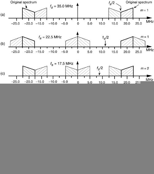
Table 2-1. Equation (2-10) Applied to the Bandpass Signal Example
|
m |
(2fc–B)/m |
(2fc+B)/(m+1) |
Optimum sampling rate |
|---|---|---|---|
|
1 |
35.0 MHz |
22.5 MHz |
22.5 MHz |
|
2 |
17.5 MHz |
15.0 MHz |
17.5 MHz |
|
3 |
11.66 MHz |
11.25 MHz |
11.25 MHz |
|
4 |
8.75 MHz |
9.0 MHz |
— |
|
5 |
7.0 MHz |
7.5 MHz |
— |
The reader may wonder, "Is the optimum sample rate always equal to the minimum permissible value for fs using Eq. (2-10)?" The answer depends on the specific application—perhaps there are certain system constraints that must be considered. For example, in digital telephony, to simplify the follow-on processing, sample frequencies are chosen to be integer multiples of 8 kHz[4]. Another application-specific factor in choosing the optimum fs is the shape of analog anti-aliasing filters[5]. Often, in practice, high-performance A/D converters have their hardware components fine-tuned during manufacture to ensure maximum linearity at high frequencies (>5 MHz). Their use at lower frequencies is not recommended.
An interesting way of illustrating the nature of Eq. (2-10) is to plot the minimum sampling rate, (2fc+B)/(m+1), for various values of m, as a function of R defined as
Equation 2-11
If we normalize the minimum sample rate from Eq. (2-10) by dividing it by the bandwidth B, we get a curve whose axes are normalized to the bandwidth shown as the solid curve in Figure 2-10. This figure shows us the minimum normalized sample rate as a function of the normalized highest frequency component in the bandpass signal. Notice that, regardless of the value of R, the minimum sampling rate need never exceed 4B and approaches 2B as the carrier frequency increases. Surprisingly, the minimum acceptable sampling frequency actually decreases as the bandpass signal's carrier frequency increases. We can interpret Figure 2-10 by reconsidering our bandpass signal example from Figure 2-7 where R = 22.5/5 = 4.5. This R value is indicated by the dashed line in Figure 2-10 showing that m = 3 and fs/B is 2.25. With B = 5 MHz, then, the minimum fs = 11.25 MHz in agreement with Table 2-1. The leftmost line in Figure 2-10 shows the low-pass sampling case, where the sample rate fs must be twice the signal's highest frequency component. So the normalized sample rate fs/B is twice the highest frequency component over B or 2R.
Figure 2-10. Minimum bandpass sampling rate from Eq. (2-10).
Figure 2-10 has been prominent in the literature, but its normal presentation enables the reader to jump to the false conclusion that any sample rate above the minimum shown in the figure will be an acceptable sample rate[6–12]. There's a clever way to avoid any misunderstanding[13]. If we plot the acceptable ranges of bandpass sample frequencies from Eq. (2-10) as a function of R we get the depiction shown in Figure 2-11. As we saw from Eq. (2-10), Table 2-1, and Figure 2-9, acceptable bandpass sample rates are a series of frequency ranges separated by unacceptable ranges of sample rate frequencies, that is, an acceptable bandpass sample frequency must be above the minimum shown in Figure 2-10, but cannot be just any frequency above that minimum. The shaded region in Figure 2-11 shows those normalized bandpass sample rates that will lead to spectral aliasing. Sample rates within the white regions of Figure 2-11 are acceptable. So, for bandpass sampling, we want our sample rate to be in the white wedged areas associated with some value of m from Eq. (2-10). Let's understand the significance of Figure 2-11 by again using our previous bandpass signal example from Figure 2-7.
Figure 2-11. Regions of acceptable bandpass sampling rates from Eq. (2-10), normalized to the sample rate over the signal bandwidth (fs/B).

Figure 2-12 shows our bandpass signal example R value (highest frequency component/bandwidth) of 4.5 as the dashed vertical line. Because that line intersects just three white wedged areas, we see that there are only three frequency regions of acceptable sample rates, and this agrees with our results from Table 2-1. The intersection of the R = 4.5 line and the borders of the white wedged areas are those sample rate frequencies listed in Table 2-1. So Figure 2-11 gives a depiction of bandpass sampling restrictions much more realistic than that given in Figure 2-10.
Figure 2-12. Acceptable sample rates for the bandpass signal example (B = 5 MHz) with a value of R = 4.5.
Although Figures 2-11 and 2-12 indicate that we can use a sample rate that lies on the boundary between a white and shaded area, these sample rates should be avoided in practice. Nonideal analog bandpass filters, sample rate clock generator instabilities, and slight imperfections in available A/D converters make this ideal case impossible to achieve exactly. It's prudent to keep fs somewhat separated from the boundaries. Consider the bandpass sampling scenario shown in Figure 2-13. With a typical (nonideal) analog bandpass filter, whose frequency response is indicated by the dashed line, it's prudent to consider the filter's bandwidth not as B, but as Bgb in our equations. That is, we create a guard band on either side of our filter so that there can be a small amount of aliasing in the discrete spectrum without distorting our desired signal, as shown at the bottom of Figure 2-13.
Figure 2-13. Bandpass sampling with aliasing occurring only in the filter guard bands.
We can relate this idea of using guard bands to Figure 2-11 by looking more closely at one of the white wedges. As shown in Figure 2-14, we'd like to set our sample rate as far down toward the vertex of the white area as we can—lower in the wedge means a lower sampling rate. However, the closer we operate to the boundary of a shaded area, the more narrow the guard band must be, requiring a sharper analog bandpass filter, as well as the tighter the tolerance we must impose on the stability and accuracy of our A/D clock generator. (Remember, operating on the boundary between a white and shaded area in Figure 2-11 causes spectral replications to butt up against each other.) So, to be safe, we operate at some intermediate point away from any shaded boundaries as shown in Figure 2-14. Further analysis of how guard bandwidths and A/D clock parameters relate to the geometry of Figure 2-14 is available in reference [13]. For this discussion, we'll just state that it's a good idea to ensure that our selected sample rate does not lie too close to the boundary between a white and shaded area in Figure 2-11.
Figure 2-14. Typical operating point for fs to compensate for nonideal hardware.
There are a couple of ways to make sure we're not operating near a boundary. One way is to set the sample rate in the middle of a white wedge for a given value of R. We do this by taking the average between the maximum and minimum sample rate terms in Eq. (2-10) for a particular value of m, that is, to center the sample rate operating point within a wedge we use a sample rate of
Equation 2-12
Another way to avoid the boundaries of Figure 2-14 is to use the following expression to determine an intermediate  operating point:
Equation 2-13

where modd is an odd integer[14]. Using Eq. (2-13) yields the useful property that the sampled signal of interest will be centered at one fourth the sample rate  . This situation is attractive because it greatly simplifies follow-on complex downconversion (frequency translation) used in many digital communications applications. Of course the choice of modd must ensure that the Nyquist restriction of
  be satisfied. We show the results of Eqs. (2-12) and (2-13) for our bandpass signal example in Figure 2-15.
Figure 2-15. Intermediate and  operating points, from Eqs. (2-12) and (2-13), to avoid operating at the shaded boundaries for the bandpass signal example. B = 5 MHz and R = 4.5.
URL http://proquest.safaribooksonline.com/0131089897/ch02lev1sec3
| Amazon | ||
