POLYPHASE FILTERS
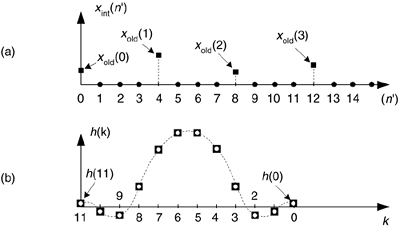
Let's assume a linear-phase FIR interpolation filter design requires a 12-tap filter; our initial plan is to pass the xint(n') sequence, Figure 10-8(a), with its zero-valued samples, through the 12-tap FIR filter coefficients shown in Figure 10-8(b), to get the desired xnew(n') sequence. (This filter, whose coefficients are the h(k) sequence, is often called the prototype FIR. That's because later we're going to modify it.) Notice with time advancing to the right in Figure 10-8(a), the filter coefficients are in reversed order, as shown in Figure 10-8(b). This filtering requires 12 multiplications for each xnew(n') output sample, with nine of the products always being zero. As it turns out, we need not perform all 12 multiplications.
Figure 10-8. Interpolation by four with a 12-tap lowpass FIR filter: (a) filter input samples; (b) filter coefficients,  's, used to compute xnew(n').
To show this by way of an example, returning to our M = 4 interpolation case, let's assume we've decided to use the 12-tap lowpass filter whose coefficients are shown in Figure 10-8(b). The job of our lowpass interpolation filter is to convolve its coefficients with the xint(n') sequence. Figure 10-9(a) shows the lowpass filter's coefficients being applied to a portion of the xint(n') samples in order to compute the first sample of xnew(n'), xnew(0). The 12 filter coefficients are indicated by the  's.
's.
Figure 10-9. Filter coefficients used to calculate various xnew(n') samples.
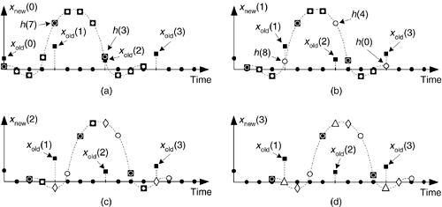
With the dots in Figure 10-9(a) representing the xint(n') sequence, we see that although there are 12  's and
  's, only the three
  's generate nonzero products contributing to the convolution sum xnew(0). Those three
  's represent FIR filter coefficients h(3), h(7), and h(11). The issue here is we need not perform the multiplications associated with the zero-valued samples in xint(n'). We only need perform 3 multiplications to get xnew(0). To see the polyphase concept, remember we use the prototype filter coefficients indicated by the
  's to compute xnew(0). When we slide the filter's impulse response to the right one sample, we use the coefficients indicated by the circles, in Figure 10-9(b), to calculate xnew(1) because the nonzero values of xint(n') will line up under the circled coefficients. Those circles represent filter coefficients h(0), h(4), and h(8).
Likewise when we slide the impulse response to the right one more sample to compute xnew(2), we use the coefficients indicated by the diamonds in Figure 10-9(c). Finally, we slide the impulse response to the right once more, and use the coefficients indicated by the triangles in Figure 10-9(d) to compute xnew(3). Sliding the filter's impulse response once more to the right, we would return to using the coefficients indicated by the  's to calculate xnew(4). You can see the pattern here—there are M = 4 different sets of coefficients used to compute xnew(n') from the xold(n) samples. Each time a new xnew(n') sample value is to be computed, we rotate one step through the four sets of coefficients and calculate as:
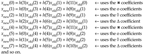
The beautiful parts here are we don't actually have to create the xint(n') sequence at all, and we perform no unnecessary computations. That is polyphase filtering.
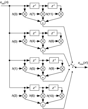
This list of calculations not only shows us what filtering to do, it shows us how to do it. We can implement our polyphase interpolation filtering technique with a bank of four sub-filters as shown in Figure 10-10. This depiction is called the commutator model for polyphase interpolation filters. We have a commutator switch rotating one complete cycle after the arrival of each new xold(n) sample. This way, four xnew(n') samples are computed for each xold(n) input sample.
Figure 10-10. Polyphase interpolation-by-four filter structure as a bank of FIR sub-filters.
In the general case, if our polyphase filter is interpolating by a factor of M, then we'll have M sub-filters. A minimum-storage structure for the polyphase filter is shown in Figure 10-11, where three commutators rotate (in unison) counterclockwise through four sets of filter coefficients upon the arrival of each new xold(n) sample. Again, four xnew(n') samples are calculated for each xold(n) sample.
Figure 10-11. Minimum-storage polyphase filter structure using commutated coefficients.
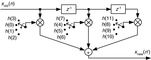
This scheme has the advantage of reducing the number of storage registers for the xold(n) input samples. If our polyphase filter is interpolating by a factor of M, then we have M sets of coefficients. We can validate our polyphase FIR filter block diagrams with z-transform equations. We start by describing our polyphase FIR filter with:

where  is a unit delay at the input sample rate, and
  is a unit delay at the output sample rate implemented with the commutator. Because
  , and
, and  , we can write:

Equation 10-6
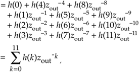
which is the classic z-domain transfer function for a 12-tap FIR filter. Equation (10-5) is called a polyphase decomposition of Eq. (10-6).
Concerning our Figure 10-9 example, there are several issues to keep in mind:
- For an interpolation factor of M, most people make sure the prototype FIR has an integer multiple of M number of stages for ease of implementation. The FIR interpolation filters we've discussed have a gain loss equal to the interpolation factor M. To compensate for this amplitude loss, we can increase the filter's coefficients by a factor of M, or perhaps multiply the xnew(n') output sequence by M.
- Our Figure 10-9 example used a prototype filter with an even number of taps, but an odd-tap prototype FIR interpolation filter can also be used[4]. For example, you could have a 15-tap prototype FIR and interpolate by 5.
- Because the coefficient sets in Figure 10-11 are not necessarily symmetrical, we can't reduce the number of multiplications by means of the folded FIR structure discussed in Section 13.7.
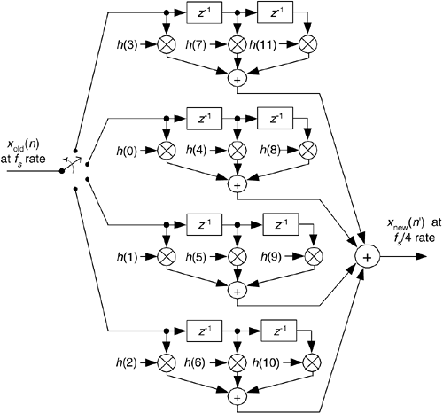
With the commutating switch structure of Figure 10-10 in mind, we can build a decimation-by-4 polyphase filter using a commutating switch as shown in Figure 10-12. The switch rotates through its four positions (D = 4), applying four xold(n) input samples to the sub-filters, then the four sub-filters' outputs are accumulated to provide a single xnew(n') output sample. Notice that the sub-filters are unchanged from the interpolation filter in Figure 10-10. The benefit of polyphase decimation filtering means that no unnecessary computations are performed. That is, no computational results are discarded to implement decimation.
Figure 10-12. Polyphase decimation-by-4 filter structure as a bank of FIR sub-filters.
In practice, large changes in sampling rate are accomplished with multiple stages (where Figure 10-12, for example, is a single stage) of cascaded smaller rate change operations of decimation and interpolation. The benefits of cascaded filters are
- an overall reduction in computational workload,
- simpler filter designs,
- reduced amount of hardware memory storage necessary, and
- a decrease in the ill effects of coefficient finite wordlength.
This introduction to sample rate conversion has, by necessity, only touched the surface of this important signal processing technique. Fortunately for us, the excellent work of early engineers and mathematicians to explore this subject is well documented in the literature.
Several standard DSP textbooks discuss these advanced multirate filter design concepts [5–7], while other texts are devoted exclusively to polyphase filters and multirate processing [8–10]. The inquisitive reader can probe further to learn how to choose the number of stages in a multistage process [1,11], the interrelated considerations of designing optimum FIR filters [1], [12], the benefits of half-band FIR filters [4,13], when IIR filter structures may be advantageous [12], what special considerations are applicable to sample rate conversion in image processing [14–16], guidance in developing the control logic necessary for hardware implementations of rate conversion algorithms [12], how rate conversion improves the usefulness of commercial test equipment [17,18], and software development tools for designing multirate filters[19].
Before concluding the subject of sample rate conversion we'll introduce one final topic, cascaded integrator-comb filters. These filters have become popular for sample rate conversion in the design of modern digital communications systems.
URL http://proquest.safaribooksonline.com/0131089897/ch10lev1sec4
 |
Amazon |  |
