DFT PROCESSING GAIN
There are two types of processing gain associated with DFTs. People who use the DFT to detect signal energy embedded in noise often speak of the DFT's processing gain because the DFT can pull signals out of background noise. This is due to the inherent correlation gain that takes place in any N-point DFT. Beyond this natural processing gain, additional integration gain is possible when multiple DFT outputs are averaged. Let's look at the DFT's inherent processing gain first.
3.12.1 Processing Gain of a Single DFT
The concept of the DFT having processing gain is straightforward if we think of a particular DFT bin output as the output of a narrowband filter. Because a DFT output bin has the amplitude response of the sin(x)/x function, that bin's output is primarily due to input energy residing under, or very near, the bin's main lobe. It's valid to think of a DFT bin as a kind of bandpass filter whose band center is located at mfs/N. We know from Eq. (3-17) that the maximum possible DFT output magnitude increases as the number of points (N) in a DFT increases. Also, as N increases, the DFT output bin main lobes become more narrow. So a DFT output bin can be treated as a bandpass filter whose gain can be increased and whose bandwidth can be reduced by increasing the value of N. Decreasing a bandpass filter's bandwidth is useful in energy detection because the frequency resolution improves in addition to the filter's ability to minimize the amount of background noise that resides within its passband. We can demonstrate this by looking at the DFT of a spectral tone (a constant frequency sinewave) added to random noise. Figure 3-22(a) is a logarithmic plot showing the first 32 outputs of a 64-point DFT when the input tone is at the center of the DFT's m = 20th bin. The output power levels (DFT magnitude squared) in Figure 3-22(a) are normalized so that the highest bin output power is set to 0 dB. Because the tone's original signal power is below the average noise power level, the tone is a bit difficult to detect when N = 64. (The time-domain noise, used to generate Figure 3-22(a), has an average value of zero, i.e., no DC bias or amplitude offset.) If we quadruple the number of input samples and increase the DFT size to N = 256, we can now see the tone power raised above the average background noise power as shown for m = 80 in Figure 3-22(b). Increasing the DFT's size to N = 1024 provides additional processing gain to pull the tone further up out of the noise as shown in Figure 3-22(c).
Figure 3-22. Single DFT processing gain: (a) N = 64; (b) N = 256; (c) N = 1024.
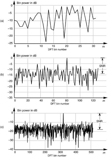
To quantify the idea of DFT processing gain, we can define a signal-to-noise ratio (SNR) as the DFT's output signal-power level over the average output noise-power level. (In practice, of course, we like to have this ratio as large as possible.) For several reasons, it's hard to say what any given single DFT output SNR will be. That's because we can't exactly predict the energy in any given N samples of random noise. Also, if the input signal frequency is not at bin center, leakage will raise the effective background noise and reduce the DFT's output SNR. In addition, any window being used will have some effect on the leakage and, thus, on the output SNR. What we'll see is that the DFT's output SNR increases as N gets larger because a DFT bin's output noise standard deviation (rms) value is proportional to  , and the DFT's output magnitude for the bin containing the signal tone is proportional to N. More generally for real inputs, if N > N', an N-point DFT's output SNRN increases over the N'-point DFT SNRN, by the following relationship:
If we increase a DFT's size from N' to N = 2N', from Eq. (3-33), the DFT's output SNR increases by 3 dB. So we say that a DFT's processing gain increases by 3 dB whenever N is doubled. Be aware that we may double a DFT's size and get a resultant processing gain of less than 3 dB in the presence of random noise; then again, we may gain slightly more than 3 dB. That's the nature of random noise. If we perform many DFTs, we'll see an average processing gain, shown in Figure 3-23(a), for various input signal SNRs. Because we're interested in the slope of the curves in Figure 3-23(a), we plot those curves on a logarithmic scale for N in Figure 3-23(b) where the curves straighten out and become linear. Looking at the slope of the curves in Figure 3-23(b), we can now see the 3 dB increase in processing gain as N doubles so long as N is greater than 20 or 30 and the signal is not overwhelmed by noise. There's nothing sacred about the absolute values of the curves in Figures 3-23(a) and 3-23(b). They were generated through a simulation of noise and a tone whose frequency was at a DFT bin center. Had the tone's frequency been between bin centers, the processing gain curves would have been shifted downward, but their shapes would still be the same,[ ] that is, Eq. (3-33) is still valid regardless of the input tone's frequency.
[
Figure 3-23. DFT processing gain vs. number of DFT points N for various input signal-to-noise ratios: (a) linear N axis; (b) logarithmic N axis.
3.12.2 Integration Gain Due to Averaging Multiple DFTs
Theoretically, we could get very large DFT processing gains by increasing the DFT size arbitrarily. The problem is that the number of necessary DFT multiplications increases proportionally to N2, and larger DFTs become very computationally intensive. Because addition is easier and faster to perform than multiplication, we can average the outputs of multiple DFTs to obtain further processing gain and signal detection sensitivity. The subject of averaging multiple DFT outputs is covered in Section 11.3.
URL http://proquest.safaribooksonline.com/0131089897/ch03lev1sec12
| Amazon | ||
