THE SLIDING DFT
The above Goertzel algorithm computes a single complex DFT spectral bin value for every N input time samples. Here we describe a sliding DFT process whose spectral bin output rate is equal to the input data rate, on a sample-by-sample basis, with the advantage that it requires fewer computations than the Goertzel algorithm for real-time spectral analysis. In applications where a new DFT output spectrum is desired every sample, or every few samples, the sliding DFT is computationally simpler than the traditional radix-2 FFT.
Table 13-4. Single-Bin DFT Computational Comparisons
|
Method |
Real multiplies |
Real additions |
|---|---|---|
|
Single-bin DFT |
4N |
2N |
|
FFT |
2Nlog2N |
Nlog2N |
|
Goertzel |
N + 2 |
2N + 1 |
13.18.1 The Sliding DFT Algorithm
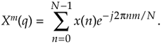
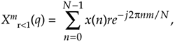
The sliding DFT (SDFT) algorithm computes a single bin result of an N-point DFT on time samples within a sliding-window. That is, for the mth bin of an N-point DFT, the SDFT computes
Let's take care to understand the notation of Xm(q). Typically, as in Chapter 3, the index of a DFT result value was the frequency-domain index m. In Eq. (13-85) the index of the DFT result is a time-domain index q = 0, 1, 2, 3, ... , such that our first mth-bin SDFT is Xm(0), our second SDFT is Xm(1), and so on.
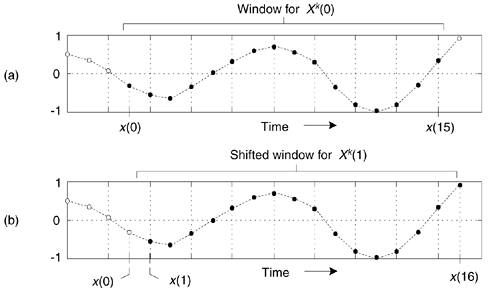
An example SDFT analysis time window is shown in Figure 13-46(a) where Xm(0) is computed for the N = 16 time samples x(0) to x(15). The time window is then advanced one sample, as in Figure 13-46(b), and the new Xm(1) is calculated. The value of this process is that each new DFT result is efficiently computed directly from the result of the previous DFT. The incremental advance of the time window for each output computation leads to the name sliding DFT or sliding-window DFT.
Figure 13-46. Analysis window for two 16-point DFTs: (a) data samples in the first computation; (b) second computation samples.
We can develop the mathematical expression for the SDFT as follows: the standard N-point DFT equation, of the mth DFT bin, for the qth DFT of the time sequence x(q), x(q+1), ..., x(q+N–1) is
Equation 13-86
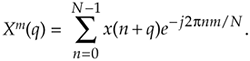
(Variable m is the frequency-domain index, where m = 0, 1, 2, ..., N–1.) Likewise, the expression for the next DFT, the (q+1)th DFT performed on time samples x(q+1), x(q+2), ..., x(q+N) , is
Equation 13-87

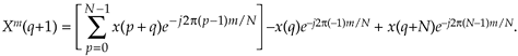
Letting p = n+1 in Eq. (13-87), we can write
Equation 13-88

Shifting the limits of summation in Eq. (13-88), and including the appropriate terms (subtract the p = 0 term and add the p = N term) to compensate for the shifted limits, we write
Equation 13-89
Factoring the common exponential term (ej2pm/N), we write
Equation 13-90
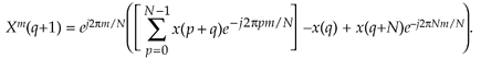
Recognizing the summation in the brackets being equal to the previous Xm(q) in Eq. (13-86), and e–j2pm = 1, we write the desired recursive expression for the sliding N-point DFT as
Equation 13-91

where Xm(q+1) is the new single-bin DFT result and Xm(q) is the previous single-bin DFT value. The superscript m reminds us that the Xm(q) spectral samples are those associated with the mth DFT bin.
Let's plug some numbers into Eq. (13-91) to reveal the nature of its time indexing. If N = 20, then 20 time samples (x(0) to x(19)) are needed to compute the first result Xm(0). The computation of Xm(1) is then
Equation 13-92

Due to our derivation method's time indexing, Eq. (13-92) appears compelled to look into the future for x(20) to compute Xm(1). With no loss in generality, we can modify Eq. (13-91)'s time indexing so that the x(n) input samples and the Xm(q) output samples use the same time index n. That modification yields our SDFT time-domain difference equation of
Equation 13-93

Equation (13-93) reveals the value of this process in computing real-time spectra. We compute Xm(n) by subtracting the x(n–N) sample and adding the current x(n) sample to the previous Xm(n–1), and phase shifting the result. Thus the SDFT requires only two real additions and one complex multiply per output sample. Not bad at all! Equation (13-93) leads to the single-bin SDFT filter implementation shown in Figure 13-47.
Figure 13-47. Single-bin sliding DFT filter structure.
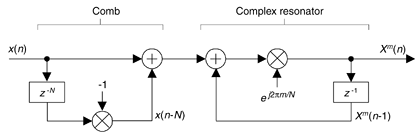
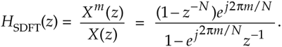
The single-bin SDFT algorithm is implemented as an IIR filter with a comb filter followed by a complex resonator. (If you need to compute all N DFT spectral components, N resonators with m = 0 to N–1 will be needed, all driven by a single comb filter.) The comb filter delay of N samples forces the SDFT filter's transient response to be N samples in length, so the output will not reach steady state until the Xm(N–1) sample. The output will not be valid, or equivalent to Eq. (13-86)'s Xm(q), until N input samples have been processed. The z-transform of Eq. (13-93) is
Equation 13-94

where factors of Xm(z) and X(z) are collected yielding the z-domain transfer function for the mth bin of the SDFT filter as
Equation 13-95
This complex filter has N zeros equally spaced around the z-domain's unit circle, due to the N-delay comb filter, as well as a single pole canceling the zero at z = ej2pm/N. The SDFT filter's complex unit impulse response h(n) and pole/zero locations are shown in Figure 13-48 for the example where m = 2 and N = 20.
Figure 13-48. Sliding DFT characteristics for m = 2 and N = 20: (a) complex impulse response; (b) pole/zero locations.
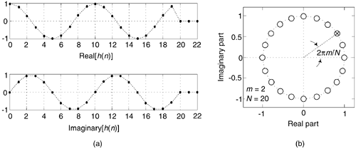
Because of the comb subfilter, the SDFT filter's complex sinusoidal unit impulse response is finite in length—truncated in time to N samples—and that property makes the frequency magnitude response of the SDFT filter identical to the sin(Nx)/sin(x) response of a single DFT bin centered at a frequency of 2pm/N.
One of the attributes of the SDFT is that once an Xm(n) is obtained, the number of computations to compute Xm(n+1) is fixed and independent of N. A computational workload comparison between the Goertzel and SDFT filters is provided later in this section. Unlike the radix-2 FFT, the SDFT's N can be any positive integer giving us greater flexibility to tune the SDFT's center frequency by defining integer m such that m = Nfi/fs, when fi is a frequency of interest in Hz and fs is the signal sample rate in Hz. In addition, the SDFT requires no bit-reversal processing as does the FFT. Like the Goertzel algorithm, the SDFT is especially efficient for narrowband spectrum analysis.
For completeness, we mention that a radix-2 sliding FFT technique exists for computing all N bins of Xm(q) in Eq. (13-85)[47,48]. That technique is computationally attractive because it requires only N complex multiplies to update the N-point FFT for all N bins; however, it requires 3N memory locations (2N for data and N for twiddle coefficients). Unlike the SDFT, the radix-2 sliding FFT scheme requires address bit-reversal processing and restricts N to be an integer power of two.
13.18.2 SDFT Stability
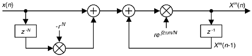
The SDFT filter is only marginally stable because its pole resides on the z-domain's unit circle. If filter coefficient numerical rounding error is not severe, the SDFT is bounded-input-bounded-output stable. Filter instability can be a problem, however, if numerical coefficient rounding causes the filter's pole to move outside the unit circle. We can use a damping factor r to force the pole and zeros in Figure 13-48(b) to be at a radius of r just slightly inside the unit circle and guarantee stability using a transfer function of
Equation 13-96

with the subscript gs meaning guaranteed-stable. (Section 7.1.3 provides the mathematical details of moving a filter's poles and zeros inside the unit circle.) The stabilized feedforward and feedback coefficients become –rN and rej2pm/N, respectively. The difference equation for the stable SDFT filter becomes
Equation 13-97

with the stabilized-filter structure shown in Figure 13-49. In this case, we perform five real multiplies and four real additions per output sample.
Figure 13-49. Guaranteed-stable sliding DFT filter structure.
Using a damping factor as in Figure 13-49 guarantees stability, but the Xm(q) output, defined by
Equation 13-98
is no longer exactly equal to the mth bin of an N-point DFT in Eq. (13-85). While the error is reduced by making r very close to (but less than) unity, a scheme does exist for eliminating that error completely once every N output samples at the expense of additional conditional logic operations[49]. Determining if the damping factor r is necessary for a particular SDFT application requires careful empirical investigation. As is so often the case in the world of DSP, this means you have test your SDFT implementation very thoroughly and carefully!
Another stabilization method worth consideration is decrementing the largest component (either real or imaginary) of the filter's ej2pm/N feedback coefficient by one least significant bit. This technique can be applied selectively to problematic output bins and is effective in combating instability due to rounding errors which result in finite-precision ej2pm/N coefficients having magnitudes greater than unity. Like the DFT, the SDFT's output is proportional to N, so in fixed-point binary implementations the designer must allocate sufficiently wide registers to hold the computed results.
13.18.3 SDFT Leakage Reduction
Being equivalent to the DFT, the SDFT also suffers from spectral leakage effects. As with the DFT, SDFT leakage can be reduced by the standard concept of windowing the x(n) input time samples as discussed in Section 3.9. However, windowing by time-domain multiplication would ruin the real-time computational simplicity of the SDFT. Thanks to the convolution theorem properties of discrete systems, we can implement time-domain windowing by means of frequency-domain convolution, as discussed in Section 13.3.
Spectral leakage reduction performed in the frequency domain is accomplished by convolving adjacent Xm(q) values with the DFT of a window function. For example, the DFT of a Hamming window comprises only three non-zero values, –0.23, 0.54, and –0.23. As such, we can compute a Hamming-windowed Xm(q) with a three-point convolution using
Equation 13-99

Figure 13-50 shows this process using three resonators, each tuned to adjacent DFT bins (m–1, m, and m+1). The comb filter stage need only be implemented once.
Figure 13-50. Three-resonator structure to compute a single Hamming-windowed Xm(q).
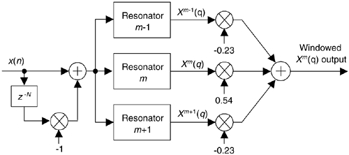
Table 13-5 provides a computational workload comparison of various spectrum analysis schemes in computing an initial Xm(n) value and computing a subsequent Xm(n+1) value.
To compute the initial windowed Xm(n) values in Table 13-5, the three-term frequency-domain convolution need only be performed once, upon arrival of the Nth time sample. However, the convolution needs to be performed for all subsequent computations
We remind the reader that Section 13.3 discusses several implementation issues regarding Hanning windowing in the frequency domain, using binary shifts to eliminate the multiplications in Eq. (13-99), as well as the use of other window functions.
Table 13-5. Single-Bin DFT Computation Comparison
|
Method |
Compute initial Xm(n) |
Compute Xm(n+1) |
||
|---|---|---|---|---|
|
Real multiplies |
Real adds |
Real multiplies |
Real adds |
|
|
DFT |
4N |
2N |
4N |
2N |
|
Goertzel algorithm |
N + 2 |
2N + 1 |
N + 2 |
2N + 1 |
|
Sliding DFT (marginally stable) |
4N |
4N |
4 |
4 |
|
Sliding DFT (guaranteed stable) |
5N |
4N |
5 |
4 |
|
Three-term windowed sliding DFT (marginally stable) |
12N + 6 |
10N + 4 |
18 |
14 |
|
Three-term windowed sliding DFT (guaranteed stable) |
13N + 6 |
10N + 4 |
19 |
14 |
13.18.4 A Little-Known SDFT Property
The SDFT has a special property that's not widely known, but is very important. If we change the SDFT's comb filter feedforward coefficient (in Figure 13-47) from a –1 to +1, the comb's zeros will be rotated counterclockwise around the unit circle by an angle of p/N radians. This situation, for N = 8, is shown on the right side of Figure 13-51(a). The zeros are located at angles of 2p(m + 1/2)/N radians. The m = 0 zeros are shown as solid dots. Figure 13-51(b) shows the zeros locations for an N = 9 SDFT under the two conditions of the comb filter's feedforward coefficient being –1 and +1.
Figure 13-51. Four possible orientations of comb filter zeros on the unit circle.

This alternate situation is useful: we can now expand our set of spectrum analysis center frequencies to more than just N angular frequency points around the unit circle. The analysis frequencies can be either 2pm/N or 2p(m+1/2)/N, where integer m is in the range 0  m N–1. Thus we can build an SDFT analyzer that resonates at any one of 2N frequencies between 0 and fs Hz. Of course, if the comb filter's feedforward coefficient is set to +1, the resonator's feedforward coefficient must be ej2p(m+1/2)/N to achieve pole/zero cancellation.
URL http://proquest.safaribooksonline.com/0131089897/ch13lev1sec18
| Amazon | ||
