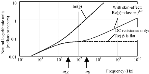
Skin-Effect Region

Beyond the LC transition the internal inductance of the conductors (a mere fraction of the total inductance) becomes significant compared to the DC resistance. This development forces a redistribution of current within the bodies of the conductors. The redistribution of current heralds the arrival of the skin-effect region (Section 3.2).

3.7.1 Boundary of Skin-Effect Region

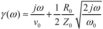
As illustrated in Figure 3.2, the skin-effect region extends to all frequencies above that point w d where the real part of the skin-effect resistance R AC [2.44] equals the DC resistance R DC [2.37].

Equation 3.103

 

where	w d is the onset of the skin-effect region (rad/s),
	k p is the proximity factor (see Section 2.10.1, "Proximity Factor"),
	k a is the DC resistance correction factor (see Section 2.4, "DC Resistance"),
	m is the magnetic permeability of the conductors (H/m),
	s is the conductivity of the conductors (S/m),
	p is the perimeter of the conductors (m), and
	a is the cross-sectional area of the signal conductor (m 2 ).
NOTE:	For differential configurations the parameters p and a are interpreted as properties of only one of the signal conductors. The constants k a and k p both assume values near two, accounting for the doubling of both DC and AC resistance due to the differential configuration. The result is that the frequency of skin-effect onset for a differential configuration occurs very nearly at the same frequency as the skin-effect onset for a single-ended configuration using one of the same physical signal conductors in juxtaposition with a solid reference plane located halfway between the two differential conductors.

If you have already computed parameters R DC and R (see Table 3.1), formula [3.103] reduces to

Equation 3.104

 

where	R DC is the DC resistance of the conductors, W /m [2.37],
	w is the frequency at which the AC line parameters are specified, rad/s, and
	R is the real part of AC resistance at frequency w , W /m [2.43].

At all frequencies above w d (including the dielectric and waveguide regions ) the skin effect plays a significant role and must be taken into account in system modeling.

The distinguishing feature of the skin-effect mode is that within this region the characteristic impedance remains fairly flat, while the line attenuation in dB varies in proportion to the square root of frequency.

POINTS TO REMEMBER

• The skin effect region starts when the internal inductance of the signal conductor becomes significant compared to its DC resistance.
• Within the skin effect region the characteristic impedance remains fairly flat, while the line attenuation in dB varies in proportion to the square root of frequency.

 

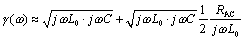
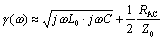
3.7.2 Characteristic Impedance (Skin-Effect Region)

The full expression for characteristic impedance ( neglecting the conductance G ) includes contributions from both the external inductance L and resistance R of the line.

Equation 3.105

 

In the limit as you proceed to frequencies far above w d (which by definition exceeds w LC ), the contribution of the term R becomes negligible, leading to this approximation for characteristic impedance in the heart of the skin-effect territory.

Equation 3.106

 

Even though in the skin-effect region R ( w ) grows in proportion to the square root of frequency, the term j w L grows faster, so that once past the crossover w LC , the contribution of R ( w ) to [3.106] is of strictly diminishing importance.

The only difference between [3.106] and the previous equation [3.85] is that here I explicitly provide for the possibility that the resistance R ( w ) may change with frequency, and the inductance term is clearly marked L to represent only the external inductance of the transmission configuration (see Section 2.7, "Skin-Effect Inductance" and Section 2.8, "Modeling Internal Impedance"). External inductance is the value of series inductance, in Henries per meter, computed by a 2-D field solver under the assumption that current rides on the surface of each conductor without penetrating its bodies.

The lumped-element , RC, and LC operating analyses presented previously assume that both L and R are constants, so it is therefore not generally necessary in those presentations to distinguish between the internal and external inductance, only lumping together all the inductance you have of either type under the umbrella term "L." Here the term from Equation [3.5] is used to represent the external inductance L e . The internal inductance of the signal conductors is represented by variations in the imaginary part of R ( w ).

As your operating frequency crosses upward from the LC to the skin-effect region, the variations in R ( w ) change (slightly) the precise shapes of the asymptotically convergent curves in Figure 3.17, but not the asymptotic points of convergence (Figure 3.27). As long as your circuit does not depend on the precise shapes of the curves, the changes have little practical significance.

Figure 3.27. The characteristic impedance of a transmission line with skin effect (solid lines) does not approach Z quite as rapidly as a line without (dashed lines).

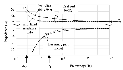
The plots starting with Figure 3.27 and going through Figure 3.30 all depict a hypothetical pcb trace having a fixed DC resistance of 6.4 W /m plus the skin effect, but no dielectric loss. The trace is a 50-ohm stripline constructed of 1/2-oz copper (17.4 micron thickness ) on FR-4 with a width of 150 microns (6 mils, v = 1.446 ·10 8 m/s, L = 346 nH/m, C = 138 pF/m). The trace is 0.5 meters long.

The general relationship between the characteristic impedance and input impedance is given by [3.33] and discussed in Section 3.5.2 "Input Impedance (RC Region)" and in Section 3.2.1 "A Transmission Line Is Always a Transmission Line."

POINTS TO REMEMBER

• At frequencies far above w d the characteristic impedance of a skin-effect limited transmission line asymptotically approaches .
• The asymptotic convergence is not quite as fast as for an LC transmission structure with fixed (non-frequency-varying) resistance.

 

3.7.3 Influence of Skin-Effect on TDR Measurement

As the skin effect increases the series resistance of a transmission line, it must also increase the degree of slope in the first TDR plateau as described under Section 3.6.3, "Influence of Series Resistance on TDR Measurements." Figure 3.28 depicts two TDR plots, the first having only a DC resistance of 6.4 W /m and the second having the same DC resistance but in addition showing the skin effect.

Figure 3.28. The AC resistance associated with the skin effect increases the slope of the initial TDR plateau.

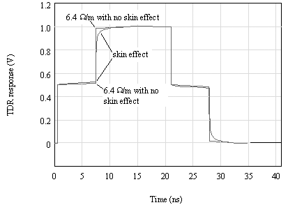
For a transmission line gripped by the skin effect, the sloping effect in the first TDR plateau begins with a slope steeper than would be predicted by the DC resistance alone. The steeper slope corresponds to the large AC (skin-effect) resistance of the line at frequencies associated with the rising edge. As time progresses the slope abates to a more moderate value corresponding to the DC resistance of the line at frequencies less than w d .

Within the skin-effect region the slope over any particular scale of time t is roughly indicated by [3.89], substituting for R DC the skin-effect resistance R AC [2.44] at a frequency corresponding roughly to 0.35/ t Hz [3.20].

For any open -circuited transmission line, [26] the second plateau of the TDR response shows a signal which has traversed the line twice, going to the far end and then reflecting back. This reflected signal displays the marks of its round-trip venture in the form of a noticeable dispersion of both rising and falling edges.

[26] The usual condition of measurement for checking the impedance of a pcb test coupon .

POINT TO REMEMBER

• The skin effect induces an upward tilt in the TDR measurement with a steep initial slope, gradually tapering to a more gentle rise.

 

3.7.4 Propagation Coefficient (Skin-Effect Region)

Figure 3.29 shows the propagation coefficient for the same hypothetical pcb trace as Figure 3.21, but this time in addition showing the skin effect (but not dielectric loss). This figure plots the real and imaginary parts of the propagation coefficient versus frequency. The plot is drawn with log-log axes to highlight the polynomial relationships between portions of the curves.

Figure 3.29. Above w d the signal loss (real part of the propagation coefficient) for a skin-effect-limited transmission line grows in proportion to the square root of frequency.

In the RC region below w LC both the real part of the propagation coefficient (log of attenuation) and the imaginary part (phase in radians) rise together in proportion to the square root of frequency. Above w LC the imaginary part (phase) grows linearly with increasing frequency, while the real part (attenuation) inflects to the right at a lesser slope. Because the skin-effect onset is so close to the LC-mode onset, the real part doesn't have sufficient room to flatten out in a true constant-loss profile. In the skin-effect region above w d the real part once again turns upward, indicating an attenuation (in dB) proportional to the square root of frequency. In this example the LC region is quite narrow, a typical result for pcb traces.

In the skin-effect region, as in the LC region, the decoupling of phase and attenuation makes it possible to construct a line with an enormous phase delay and yet very low attenuation. Terminations are used within the skin-effect region to abate resonance on long transmission lines in precisely the same manner as used in LC region.

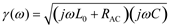
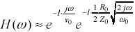
You can predict the phase and amplitude response of a skin-effected transmission line beginning with the definition of the propagation function [3.13], assuming operation at a frequency well in excess of w d so that R AC >> R DC .

Equation 3.107

 

where

L represents the external inductance and where information about the internal inductance is coded into the imaginary part of R AC .

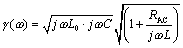
Factor out the common j w L and j w C terms.

Equation 3.108

 

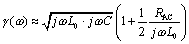
Assuming you are dealing at a frequency well in excess of w LC so that j w L >> R AC , you may linearize the second square-root:

Equation 3.109

 

and distribute the first term into the second:

Equation 3.110

 

Combine all the L and C elements in the right-hand term, and make the substitution :

Equation 3.111

 

On the right, substitute your assumption [2.50] about R AC , and on the left factor j w out of the square root:

Equation 3.112

 

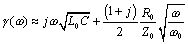
What remains is a linear-phase term , representing the bulk transport delay of the transmission-line medium, and a low-pass filter term whose attenuation in dB grows in proportion to the square root of frequency. [27]

[27] Remember that the real part of the propagation coefficient shows the attenuation in nepers. Increasing attenuation at high frequencies indicates a low-pass filtering effect, decreasing the propagation function H (see [3.14]).

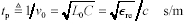
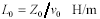
The linear-phase term implies that the one-way propagation function H of a skin-effect-limited transmission line, for frequencies above w d , acts as a large time-delay element. The bulk propagation delay in units of seconds per meter is given by

Equation 3.113

 

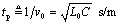
Equation [3.113] may also be stated in terms of the effective relative permittivity re associated with the transmission line configuration , assuming the speed of light c = 2.998 ·10 8 m/s and further assuming the relative magnetic permeability m r equals unity (see [2.28]).

The overall bulk transport delay for a transmission line varies in proportion to its length. Doubling the length doubles the bulk transport delay.

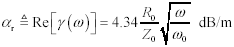
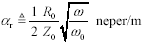
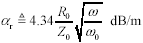
The transfer loss in nepers per meter is given by the real part of the propagation function. This value is called the skin-effect loss coefficient :

Equation 3.114

 

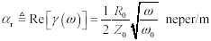
Equation 3.115

 

The low-pass filtering action of the skin effect implies that the step response will be dispersed, slurring crisp rising edges into edges of limited rise and fall time, according to the properties of the filter.

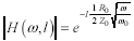
The magnitude of H is determined from the real part of the propagation function (see [2.16]):

Equation 3.116

 

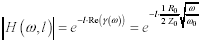
where	H ( w ,l ) is the magnitude of the low-pass filter function implied by [3.112],
	l is the length of the transmission line in meters,
	w is the frequency at which AC line parameters are specified, rad/s,
	R is the AC resistance of the line at frequency w , and
	Z is the characteristic impedance of the line at frequency w .

The signal loss represented by H , measured in nepers (or decibels), varies in proportion to the length of the transmission line and in proportion to the square root of frequency. Double the distance yields twice the loss in neper or decibel units (one neper equals 8.6858896 dB). Doubling the frequency multiplies the loss (in neper or dB units) by the square root of two.

Binary signaling tolerates a tilt of no more than about 3 dB (and certainly never more than 6 dB) in the channel attenuation over the band occupied by the coded data. Any tilt greater than that amount must be flattened out with an equalizer (see Section 3.14, "Linear Equalization: Long Backplane Trace Example").

Be careful with your units conversions when calculating attenuation, as the data rate f for most systems is expressed in Hertz, while the frequency argument for the function H ( w ) is specified in radians per second. You must multiply f by 2 p to get w .

The properties in Table 3.6 hold only for transmission lines operated at frequencies well above the skin-effect onset w d but below the onset of the dielectric loss region. Subsequent sections discuss the implications of dielectric loss, which further increases line attenuation.

Table 3.6. Summary of Skin-Effected-Limited Transmission Line Properties at Frequencies Well Above w d

Property	Formula	Ref. equation
Asymptotic value of characteristic impedance		[3.106]
Bulk transport delay per meter [1]		[3.113]
Attenuation in nepers per meter (1 neper = 8.6858896 decibels)		[3.114]
Attenuation in decibels per meter		[3.115]
Transfer gain at length l		[3.116]
Inductance per meter		[3.5]
Capacitance per meter		[3.6]

[1] NOTE (1) ”TIA/EIA 568-B specifications suggest following more detailed approximation for phase delay on long cables operated within the skin-effect limited region: . This expression may be derived from [3.116]. A related expression exists for group delay within the skin-effect limited region: .

POINTS TO REMEMBER

• The attenuation (in dB) within the skin-effect region grows in proportion to the square root of frequency.
• Doubling the length of a skin-effect-limited transmission line doubles the attenuation.

 

3.7.5 Possibility of Severe Resonance within Skin-Effect Region

Transmission lines operated in the skin-effect region fall prey to the same resonance difficulties that afflict structures operated in the LC region. The termination means used to conquer resonance are the same as those described in Section 3.6.6, "Terminating an LC Transmission Line."

One difference, however, between the severity of resonance associated with a pure LC structure and the severity of the resonance associated with a skin-effect-limited structure has to do with the additional attenuation present due to the skin effect. In the equation for overall system gain G , the height of the resonant peaks is determined by the depth of the cancellation in the denominator. If the magnitude of the one-way propagation function H evaluated at the frequency of resonance indicates a substantial amount of attenuation, then the magnitude of the term H 2 G 1 G 2 can never approach unity, and the resonance will fail to materialize.

In the frequency domain the skin effect causes a lessening of the heights of the resonant peaks in Figure 3.22, with the heights (in dB) of higher resonant modes falling off inversely with the square root of frequency.

In practice it is impossible to incorporate into a transmission structure sufficient internal loss to satisfactorily limit the resonance (i.e., reflections) while also providing a reasonably clean, full- sized signal at the far end of the structure. The skin-effect losses do, however, have the beneficial effect of reducing (somewhat) the requirements for efficacy of the intentional termination placed in the circuit.

Example of Limitation on Size of Resonance

Suppose on an open-circuited line of length 0.1 meter (3.9 in.) the first resonance f 1 = l /(4 v ) occurs at 754 MHz. Further assume that at that frequency the magnitude of H ( w ) equals 1/2 (i.e., “6 dB.). The magnitude of H 2 G 1 G 2 therefore cannot exceed 1/4, and the worst-case resonance therefore will not exceed 1/(1 - 1/4) = 4/3, or about 33% overshoot.

I should caution you against the wisdom of designing any system whose proper operation depends upon some "minimum attenuation" within the interconnections. It is quite possible that while your system as it is implemented today may enjoy the benefits of a minimum amount of attenuation within every interconnection, this property may not be true in the future, particularly if the technology used to construct the interconnections is upgraded. One excellent class of examples of systems that have been designed assuming some minimum attenuation, and then rendered less robust by the use with a lower-attenuation class of cabling, would be those LAN systems designed for use with category-III unshielded twisted-pair cabling. This cabling infrastructure was upgraded in many companies beginning in 1995 to a newer , lower-attenuation form of supposedly backwards -compatible cabling called category-5 unshielded twisted-pair cabling.

Another good example would be transceivers designed for FR-4 pcb substrates that may someday be used in systems with low-dielectric loss substrates like Getek.

As a final example, the original T1 connections deployed by the telephone company depended upon a minimum attenuation property. In the original version of that system each line was padded by hand, using special circuitry to guarantee a consistent line loss (and frequency response) independent of line length on every wire pair. The receivers therefore could incorporate a large fixed gain without concern for overloading. That sort of hand tweaking and testing on every individual wire pair is no longer economically feasible .

3.7.5.1 Subtle Differences Between Termination Styles

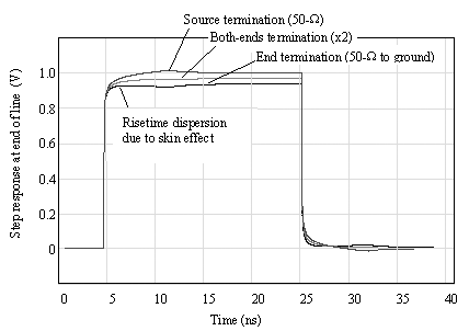
Figure 3.25 is repeated here showing the inclusion of skin-effect losses (Figure 3.30). All three traces clearly show dispersion of the rising and falling edges caused by the low-pass filtering properties of the skin-effect resistance.

Figure 3.30. Different termination styles react differently to skin-effect resistance.

3.7.5.2 Application of Termination Equations to Other Regions

The LC, skin-effect, and dielectric-loss-limited regions all share the same asymptotic high-frequency value of characteristic impedance Z . The same termination approaches therefore work for all three regions, delivering in each case an overall circuit gain G nearly equal to the one-way propagation function H applicable within each region.

POINT TO REMEMBER

• Transmission lines in the skin-effect region fall prey to the same resonance difficulties that afflict the LC region and respond to the same means of termination.

 

3.7.6 Step Response (Skin-Effect Region)

This section presents the step response of a skin-effect-limited transmission line. The applicability of these results hinges on two crucial assumptions:

1. The risetime of the step input to the system must be substantially faster than the skin-effect risetime (meaning that the shape of the output waveform is determined primarily by the system itself and not strongly influenced by the precise risetime of the input step), and
2. The impedance of the line's series inductance greatly exceeds its series resistance (so that you have a true low-loss transmission media and not an RC dispersion line).

The solution requires knowledge of these parameters:

• Z , the nominal characteristic impedance of the transmission line at high frequencies (excluding the effect of the internal inductance of the wires), in ohms,
• w , some particular frequency at which the skin-effect resistance is specified (rad/s),
• R , the series skin-effect resistance ( W /m) at frequency w , and
• l , the length of the line (m).

Beginning with [3.112], substitute 1/ v for the radical and make the substitution .

Equation 3.117

 

Multiply the result by the (negative of the) transmission line length l and exponentiate (as in [3.14]) to find H .

Equation 3.118

 

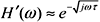
The first exponential term in [3.118] represents a linear-phase bulk transport delay. This delay, for the purposes of investigating attenuation and dispersion of the propagated signals, may be ignored. The second exponential term encodes the low-pass filter function associated with the skin effect. Call this filter H '( w ). Normalize H '( w ) by substituting into it the arbitrary constant .

Equation 3.119

 

To compute the step response of the skin effect numerically , multiply [3.119] by 1/ j w and then apply an inverse Fourier transform. Multiplying by 1/ j w converts [3.119] from an impulse-response to a step-response. Evaluating the inverse Fourier transform of the result produces a time-domain waveform that represents the step response of the skin effect.

The following well-known Fourier transform pair accomplishes the calculation of the skin-effect step response. [28] , [29]

[28] The author has been informed that a trivial variant of this transform pair is found in the 10th edition of the CRC Handbook of Chemistry and Physics , in the table of transforms, item number 84, although not in more modern editions of this book. The transform pair is also found in the appendix of R.V. Churchill's text Operational Mathematics , 3rd edition, also denoted 84. A more modern reference is found in the Table of Integrals, Series and Products , 5th ed., 1994 (translated from Russian) by Gradshteyn and Ryzhik, although in their listing they call out the use of the function erf( ) instead of erfc( ), which appears to be a mistake.

[29] The identification of the step response associated with the skin effect was first made by R. L. Wigington and R. S. Nahman, "Transient analysis of coaxial cables considering skin effect," Proc. IRE, vol 45, pp. 166 “174; Feb. 1957. Their work was conducted in the context of the development of nuclear instrumentation for test-blast monitoring. The specific problem at hand had to do with whether signals from the blast sensors could travel down a coaxial cable to the test shack faster than the radiant wave of heat from the blast vaporized the cable.

Equation 3.120

 

where	u ( t ) is the unit step function, equal to one for all t 0 and zero otherwise ,
	erfc ( ) is the complementary error function, defined in Appendix E.
	the symbol represents an inverse Fourier transformation, and
	t may take on any positive value.

The normalized skin-effect time-and-frequency-response transform pair illustrated in Figure 3.31 conforms exactly to equation [3.120] with parameter t = 1. The top two figures show the magnitude of the propagation function (in dB) of a long, perfectly terminated skin-effect-limited channel. The bottom two figures show the step response of the channel, one with a logarithmic time scale, the other with a linear timescale .

Figure 3.31. The step response associated with the skin effect has a quick rise and a long, sloping tail.

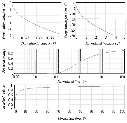
Assuming you have calculated the value t used in [3.119], you may read from these charts directly the frequency response (magnitude) and step response (assuming a normalized 1-volt step input with zero risetime) for any skin-effect-limited system.

Table 3.7 presents selected values from the charts in Figure 3.31. Two rules of scaling apply to the quantities in this table:

1. The relative ratios among the time-domain measurements listed apply equally to any skin-effect-limited channel.
2. The product of any time-domain measure and any frequency-domain measure (for example, T 10-90% · F 3dB ) remains constant for any skin-effect-limited channel.

Notice that the skin effect acts over a very wide scale of times. At the beginning of the step response, the slope is very sharp. Towards the end, the step response has a long, slow-moving tail. Any equalizing circuit built to undo the skin effect must be capable of producing subtle variations in its propagation function over a correspondingly wide range of frequencies.

The long settling time of the skin-effect phenomenon has serious implications for testing. Any measurement setup used to research skin-effect behavior must provide enough time for the skin-effect response to fully settle to 99% or more of its final value. Experiments involving truncated step-response waveforms will be missing significant portions of the overall step response waveform and will not reproduce the same risetime ratios as predicted in Table 3.7.

Table 3.7. Selected Values of Skin-Effect Step Response

Percentile point	Time to achieve (s)
T 10	0.1848 t
T 20	0.3044 t
T 47.9500	1.0000 t
T 50	1.0990 t
T 80	7.7900 t
T 90	31.6643 t
T 95	127.159 t
T 97	353.52 t
T 98	795.63 t
T 99	3183.03 t
Attenuation point	Frequency at which point is reached (Hz)
F- 3dB	0.0379/ t
F- 6dB	0.1518/ t

Similarly, bit-error-rate measurements taken with a pseudorandom pattern insufficiently long to exercise the full range of skin-effect behavior will return overly optimistic results.

Example of Insufficiently Long Pseudorandom BER Test

The skin-effect band for Belden type 8237 coaxial cable extends from 24 KHz to 5.9 GHz. Suppose you are working with a section of this cable whose length creates a skin-effect risetime of T 50 = 1 ns. How long does the step response take to reach 99% of full value? In Table 3.7 the ratio T 99 / T 50 is 3183/1.099; therefore, the time to reach 99% is (3183/1.099) ·(1 ns), which equals 2896 ns.

If the system bit time is 100 ns (10 Mb/s), then it takes (in theory) 29 bits for the skin-effect step response to reach 99% of its full value. A good pseudorandom BER test should therefore include a pattern with at least 29 bits in a row held low, followed by a transition, and at least 29 bits in a row held high, followed by a transition. This would seem to indicate a need for at least a 29-bit pseudorandom pattern generator.

A 7-bit (128-length) pattern generator holds at most 7 bits in a row high or low, at which point the skin-effect response progresses to only 97% or 98% of its final value, leaving untested the final 2% to 3% of intersymbol interference (ISI).

The value t associated with [3.119] and [3.116] varies with the square of distance; therefore, the risetime of a skin-effect-limited channel scales with the square of its length. To see the relation directly, substitute the definition of t into the expression in Table 3.7 for T 50 .

Equation 3.121

 

where	w is the particular frequency at which the skin-effect resistance is specified (rad/s),
	l is the length of the line (m),
	R is the series skin-effect resistance ( W /m) at frequency w , and
	Z is the nominal characteristic impedance of the transmission line at high frequencies (excluding the effect of the internal inductance of the wires), ( W ).

The square of length is a very fast-changing function. If you cut in half the length of a skin-effect-limited transmission channel, you decrease its risetime fourfold. Cutting the length to 1/10 shortens the risetime by a factor of 100.

The skin-effect risetime also scales with the square of R , which is inversely proportional to the perimeter of the signal conductor. Therefore, a conductor twice the diameter (or width) has 1/2 the AC resistance and 1/4 the skin-effect risetime. This scaling principle explains the tremendous bandwidth advantages of large coaxial cables. It also makes clear that the difference in skin-effect risetime between a 75-micron (3-mil) trace and a 150-micron (6-mil) trace is a factor of four.

Beware that the skin-effect and dielectric-loss effects mix together over a very broad range of frequencies. It's rare in pcb problems that you see skin-effect losses without also having to take into account dielectric dispersion. The best general rule for combining dispersion due to different sources is the sum-of-squares rule, which works as follows .

Equation 3.122

 

If you seek a more exact answer, take the skin-effect and dielectric-loss impulse responses outlined in this and the next section and convolve them together. Or better yet, use the complete frequency-domain model from the previous chapter, sample it on a dense grid of frequencies, and inverse-FFT to get the complete time-domain step response.

POINT TO REMEMBER

• The step response associated with the skin effect has a quick rise and a long, sloping tail.

 

3.7.7 Tradeoffs Between Distance and Speed (Skin-Effect Region)

Given a fixed receiver architecture, and assuming the BER of the receiver is dominated by errors due to intersymbol interference, the speed of operation within the skin-effect region scales inversely with the square of transmission-line length. This tradeoff between length and speed arises because the distributed skin effect produces attenuation (in dB) proportional to the square root of frequency. For example, a 10% increase in length increases the attenuation (in dB) by 10%. To regain a normal signal amplitude at the end of a transmission line limited by skin-effect losses, the 1% increase in attenuation may be offset by a 20% reduction in the system operating speed.

POINTS TO REMEMBER

• The risetime of a skin-effect-limited channel scales with the square of its length.
• The speed of operation within the skin-effect region scales inversely with the square of transmission-line length.
• A conductor twice the diameter (or width) has 1/4 the AC resistance and thus 1/4 the skin-effect risetime.
• It's rare in pcb problems that you see skin-effect losses without also having to take into account dielectric dispersion.