Miscellaneous Problems | Part III - Advanced Problems in Data Structures

Table of contents:

PROBLEM THE TWO CLASS CLASSIFICATION PROBLEM

Given a training data set having two classes and the functional form of the decision boundary between them, find the decision boundary of that form that best separates the two classes. Assume that a linear decision boundary will be used to classify samples into two classes, and that each sample has M features.

Program

#include typedef enum {FALSE, TRUE} boo1 ; int computeD(int *x, int n, int Jw) { /* * compute the value of the discriminant function D using the xis and wis. * D = w0 + w1x1 + w2x2 + ... + wnxn. */ int i; int d = w[0]; for(i=l; i<=n; ++i) d += w[i]*x[i]; return d; } int signum(int d) { /* * signum(d) = 1 if d>=O * = -1 otherwise. */ if(d = 0) return 1; return -1; } void updateW(int *x, int n, int *w, const int c, const int k, int d) { /* * update the ws as the discriminant function was different than the class * value. * wi += cdxi for l<=i<=n. * w0 += cdk. */ int i; w[0] += c*d*k; for(i=l; i<=n; ++i) w[il += c*d*x[il; } void printHeader(int n) { /* * print header of the output */ int i; for(i=l; i<=n; ++i) printf ("x%d ", i) ; printf ("d "); for(i=0; i<=n; ++i) printf("old w%d ", i) ; printf("D Error? ") ; for(i=0; i<=n; ++i) printf("new w%d ", i); printf (" "); } int findK(FILE *fp, int n) { int tempk, k=0, count=0; int i; while(fscanf(fp, "%d", &tempk) == 1) { // x1. k += tempk; for(i=2; i<=n; ++i) {// x2 to xn. fscanf(fp, "%d", &tempk); k += tempk; } fscanf(fp, "%d", &tempk); // d. count++ ; } k /= count*n; k = abs(k); return k; } void printArray(int *xorw, int n) { /* * print xorw[0. .n-1]. */ int i; for(i=0; i

Explanation

If the discriminant function is of the form D = w0 + w1x1 + … + wMxM, then D = 0 is the equation of the decision boundary between the two classes. The weights w0, w1, …, wM are to be chosen to provide good performance on the training set. A sample with feature vector x = (x1, …, x2) is classified into one class, say class 1 if D >= 0, and into the other class, say class −1 if D < 0. Geometrically, D = 0 is the equation of a hyperplane decision boundary that divides the M-dimensional feature space into two regions. Two classes are said to be linearly separable if there exists a hyperplane decision boundary such that D > 0 for all the samples in class 1, and D < 0 for all the samples in class −1.
The adaptive decision boundary algorithm consists of the following steps:
2. Initialize the weights w0, …, wM to zero or to small random values or to some initial guesses. Choosing good initial guesses for the weights will speed convergence to a perfect solution if one exists.
4. Choose the next sample x = (xl, …, xM) from the training set. Let the true class of desired value of D be d, so that d = 1 or −1 represents the true class of x.
6. Compute D = w0 + w1x1 + … + wMxM.
8. If signum(D) != d, replace wi by wi + cdxi, for i = 1, …, M, where c is a positive constant that controls the step size for weight adjustment. signum(D) == 1 if D >= 0 and signum(D) == −1 if D < 0. Also replace w0 by w0 + cdk where k is a positive constant. If signum(D) == d, then no change in the weights should be made. We take k to be the average absolute value of all the features for fast convergence.
10. Repeat steps b through d with each of the samples in the training set. When finished, run through the entire training data set again. Stop and report perfect classification when all the samples are correctly classified during one complete pass of the entire training set through the training procedure. An additional stopping rule is also needed since this process would never terminate if the two classes were not linearly separable. A fixed maximum number of iterations could be tried, or the algorithm could be terminated when the running average error rate ceases to decrease significantly. We assume that the classes are linearly separable.
The data is read from a file. The first line of the file should contain a single number n signifying the number of features. From line 2 onwards, each line contains n+l numbers representing one sample. It contains n feature values followed by the class value (1 or −1). One pass of the file is done in findK() to find the average absolute value of the features to be assigned to the constant k for fast convergence to the solution, if it exists. main() then contains a loop that runs as long as there is at least one misclassification in the whole data set. The inner while loop reads every sample and stores the vector x in an array x[] from indices 1 to n. x[0] stores the class value d. w[0 . . n] is another array that stores the values of weights w0, …, wn. Initially, all ws are set to zero. The function computeD() computes the value of the discriminant function D by using x[] and w[]. We then check whether signum(D) == class value d. If they are equal, nothing is done; otherwise, w[] vector is changed as given in the preceding algorithm. The function printArray() prints a vector.

Example: Let the training file be 1 −4 −1 −1 1. This means there is only one feature and there are two samples. In the first, the value of x1 is −4 and its class is −1. The second contains the value of x1 as −1, and its class is 1. Let c = 1. k = average absolute value of features = abs((−4−1)/2) = abs(−2) = 2. w0 = w1 = 0. Using the first sample x1 = −4 results in D = w0 + w1x1 = 0 + 0(−4) = 0, where we have arbitrarily assigned the sign of 0 to be 1. However, d = −1, so the sample is misclassified and we adapt the weights as follows: W0 = W0 + cdk = 0 + 1(−1)2 = −2. w1 = w1 + cdx1 = 0 + 1(−1)(−4) = 4. The algorithm is repeated until both samples are correctly classified. Different steps of the algorithm are as follows:


step	x1	d	old w0	old w1	D	Error?	new w0	new w1





1	−4	−1	0	0	0	yes	−2	4

2	−1	1	−2	4	−6	yes	0	3

3	−4	−1	0	3	−12	no	0	3

4	−1	1	0	3	−3	yes	2	2

5	−4	−1	2	2	−6	no	2	2

6	−1	1	2	2	0	no	2	2

Points to Remember

One way to assure a sort of convergence, even when the classes are not linearly separable, is to replace the constant c by a variable step size that decreases with the number of iterations. However, convergence to a decision boundary that best separates the classes is not guaranteed when the classes are not linearly separable.
Nonlinear decision boundaries that are more complex than hyperplanes can also be found by this adaptive technique.
If there are more than two classes, but each pair of classes is linearly separable, then the same algorithm can be used to find the boundary between each two pairs of classes.

PROBLEM THE N COINS PROBLEM

Given a string of 0s and 1s as tails and heads obtained from tossing n coins of arbitrary biases, find the (approximate) points where the change of coin could have taken place.

Program

#include 
#include 

#define MINGROUPSIZE 10
#define EPSILON 0.08

int adjustPartition(int *a, int n, double *p, int m, int i) {
 /*
 * slide the partition boundary from i forward or backward to get
 * better partition and return the index of the last element in the
 * partition.
 * i >= 1.
 */
 int aindex = i*MINGROUPSIZE;
 int j, startj = aindex-MINGROUPSIZE/4, finalj = aindex+MINGROUPSIZE/4 ;
 int k;
 int ones, nelem;

 for(k=(i - l)*MINGROUPSIZE, nelem=0; k= EPSILON) // found the partition.
 break;
 }
 return j;
}

int findChange(int *a, int n, double *p, int m) {
 /*
 * the running probabilities are given in p[m].
 * find the points of coin change from them.
 */
 int i;
 for(i=l; i= EPSILON) // found the change.
 return adjustPartition(a, n, p, m, i);
 }
 return -1;
}

int findProb(int *a, int n, double *p) {
 /*
 * find the average probabilities of groups in a[n] and store in p.
 */
 int i, j=-1, k, ones, nelem;

 for(i=0; i−1) {
 printf("partiti0n at %d.
", startoff+partindex) ;
 printAverage(a, partindex);
 findPartition(a+partindex, n − partindex, p, startoff+partindex);
 }
 else
 printAverage(a, n);
}
int main() {
 int a[] = {0,0,0, 1,0,0,0,1,1,1,1,1,0,1,1,1,1,0,0, 0,0,1,0,0,1,0,0,0,1,0};
 double *p;
 int n = sizeof(a)/sizeof(int);
 int m;

 p = (doubl e *)ma1 1 oc((n+MINGROUPSIZE − 1) / MINGROUPSIZE*sizeof(double);
 findPartition(a, n, p, 0);

 return 0;
}

Explanation

Consider the following input string:
```
0,0,0,1,0,0,0,1,1,1,1,1,0,1,1,1,1,0,0,0,0,1,0,1,0,0,0,1,0,0,1,0,0,1,0,0,0,1,0.
```
Visually, we may partition it as follows:
```
0,0,0,1,0,0,0 1,1,1,1,1,0,1,1,1,1 0,0,0,0,1,0,1,0,0,0,1,0,0,1,0,0,1,0,0,0,1,0.
```
We define bias of a coin as the probability of tossing a head (1).
Thus, bias of coin 1 = 1/7 = 0.14.
bias of coin 2 = 9/10 = 0.9.
bias of coin 3 = 6/22 = 0.27.

Thus, we have to find such partitions in the input string.

Note two extreme cases. First, there was a single coin whose bias is 16/39 = 0.41. Second, there were 39 coins with biases equal to their outcomes (0 or 1). These conclusions are valid but of no practical importance. What we are interested in are patterns of 0s and 1s that appear uniformly over a length of the string.
Since this is a problem with an approximate solution, there can be various ways to get an answer. We have chosen the following strategy. We partition the elements (0s and 1s) into various groups of a fixed size MINGROUPSIZE (perhaps except the last group) and find the average biases of each group. We then compare adjacent group biases, and if the difference in the biases is >= an error term EPSILON, we know that these two partitions have different patterns, and so a possible change of coin took place somewhere near the boundary between the two partitions. We then try to shift the boundary by some fixed amount and find a suitable partition point. Thus, we found out one possible change of coin. We run this algorithm recursively to find the next partitions in the input.
The function findPartition() is the driver function. It calls findProb() to group the elements of the input string into various partitions and find their average biases. It then calls findChange() to check whether there are consecutive biases having a difference of >= EPSILON. The function findChange() returns −1 if there is no such change. Otherwise, it calls adjustPartition() to make a smooth change to the partition index for better accuracy. The function adjustPartition() slides the end of the partition from -MINGROUPSIZE/3 to 0 to +MINGROUPSIZE/3 across the original boundary and stops as soon as the difference in the biases of the original partition and the sliding partition is >= EPSILON. The function printAverage() is a dummy function used to print values required for understanding and debugging.
Example: Let MINGROUPSIZE=10 and EPSILON=0.08.

For this input string, the function findProb() groups the elements into the following partitions having the given biases:
group 0 = 0,0,0,1,0,0,0,1,1,1 bias = 4/10 = 0.4.
group 1 = 1,1,0,1,1,1,1,0,0,0 bias = 6/10 = 0.6.
group 2 = 0,1,0,1,0,0,0,1,0,0 bias = 3/10 = 0.3.
group 3 = 1,0,0,1,0,0,0,1,0 bias = 319 = 0.33.

The first call to findChange() tells that there is a change of >= EPSILON between group 0 and group 1. Thus, the partition wall is assumed between the two groups. This wall is shifted from its position from negative to positive direction in the function adjustPartition(). The offset within which this is done is fixed at MINGROUPSIZE/4. If the difference between the average bias of the partition before this wall and the average bias of the partition before the original partition wall becomes >= EPSILON, then the partition wall is fixed at that point.

Thus the first partition is fixed at index 8, and is 0,0,0,1,0,0,0,1 with average bias of 2/8 = 0.25.

The remaining array is then partitioned recursively in a similar manner. Thus we get the remaining partitions as 1,1,1,1,0,1,1,1 with average bias of 7/8 = 0.88 and 1,0,0,0,0,1,0,1,0,0,0,1,0,0,1,0,0,1,0,0,0,1,0 with average bias of 7/23 = 0.3.

Points to Remember

One can find an input string that can fool this algorithm for a fixed group size MINGROUPSIZE and error term EPSILON.
There will be greater accuracy if some adaptive algorithm is used that will refine the partitions.
This algorithm can be used in noise detection and correction of the input signal.

PROBLEM ALL COMBINATIONS OF STRINGS

Write a program to print all the combinations of a string.

Program

#include #define MAXLEN 80 void init(char *answer, int slen) { /* * initialize first slen entries in answer[] to 0. */ int i; for(i=O; i

Explanation

Consider an input string abc. Various combinations of this string are abc, acb, bac, cab, bca, and cba. To generate these combinations, we once again make use of recursion.
Note that combinations of the string "abc" are obtained by fixing character ‘a’ at different positions and finding combinations of string ‘bc’. Fixing ‘a’ at a position means, in the answer string, the character ‘a’ will occur at a fixed position. Similarly, combinations of string ‘bc’ can be found by fixing character ‘b’ at different positions and finding combinations of string ‘c’. If string ‘c’ has only one combination, we get the following:
```
comb('c') = c.
comb('bc') = bc /* character 'b' fixed at position 1. */
 and cb /* character 'b' fixed at position 2. */
comb('abc') = a fixed at different places in comb('bc').
 = abc and acb /* character 'a' fixed at position 1. */
and bac and cab /* character 'a' fixed at position 2. */
and bca and cba /* character 'a' fixed at position 3. */
```
The program repeatedly asks for a string until the entered string is empty and calls printComb(). printComb() fixes the position of a character and calls printComb() recursively for the remaining string.
The complexity of printComb() can be easily derived from the following recurrence relation:

T(n) = n*T(n−1).

This is because, for finding combinations of a string of length n, we fix the position of a character at a position out of n possible positions and then find combinations of the remaining (n−1) characters. After solving the equation, we get the complexity of printComb()1 as O(n!).

Points to Remember

The complexity of printComb() is O(n!) where n is the length of the input string .
A simple recursive procedure, such as printComb(), can solve a larger problem in an elegant manner.
Care should be taken to end a string with ‘O’, as done in function init().

PROBLEM THE 8 KNIGHTS PROBLEM

Solve the problem of a knight's tour without backtracking. Assume that it starts from a corner of the chessboard.

Program

#include #define M 8 #define NDIR 8 // no of directions. typedef enum {FALSE, TRUE} boo1 ; int rowchange[] = {−2, −1, 1, 2, 2, 1, −1, −2}; int colchange[] = {−1, −2, −2, −1, 1, 2, 2, l}; void printMatrix(int a[][M], int n) { /* * print the final solution. */ int i, j; for(i=O; i=0 && row=0 && newrow=0 && newcol−1; int i; a[row][col] = num; if(num = n*n) return; for(i=O; i−1, num+l); } int main() { int a[M][M] ; //here you have to initialize matrix int i=0, j=0; for(i=0; i

Explanation

On an 8 × 8 chessboard, a knight can travel two-and-a-half positions at a time. The problem is to start from a corner of the chessboard and visit all 64 positions without visiting any position more than once. This travel is called a knight's tour.
There is more than one way to solve this problem. We implement here the strategy suggested by J.C. Warnsdorff in 1823. His rule is that the knight must always be moved to one of the positions from which the minimum number of not-yet-visited positions can be traversed.
The knight can visit one of the eight (at most) positions from a fixed position. Those are shown in Figure 29.1. It is possible that the number of positions that can be traversed is less than eight, depending on the chessboard boundaries and visit of the knight to other squares.

Figure 29.1: A knight can move to a maximum of eight positions.

If the board is represented (naturally) by 8x8 matrix of integers a[8] [8], and if the current position of the knight is a[i][j], then the next position could be one the eight: a[i−2][j−1], a[i−1][j−2], a[i+1][j−2], a[i+2][j−1], a[i+2][j+1], a[i+1][j+2], a[i−1][j+2], a[i−2][j+l]. We maintain two arrays of these changes in row and column in rowchange[8] and col change[8]. Thus, if the current position is a[i][j], then the next position in direction d, l<=d<=8, as shown in the figure, is given by a[i+rowchange[d−l]][ j+colchange[d−1]].
The program initializes the array by zeros and calls function knight() with the values of (row. column) as (0, O), which forms the first position of the knight. Then, for each of the eight directions we find the new position a[newrow][newcol] using the rule in Number 3. From each of these entries, we find the number of positions to which the knight can travel (getCost()). We select the minimum of such values and call knight() recursively for that position and so on until we finish all the squares. As we visit a position, we mark it to print the path at the end of the traversal.

Points to Remember

The knight's tour can be solved with backtracking by the trial-and-error method in which we select the next move randomly, and, if we find it to be non-feasible, we backtrack and try another direction. Its complexity is exponential.
The problem of the knight's tour can also be solved without backtracking in O(N × N) time where N is the size of the chessboard.
There are other heuristics available that can solve the problem of the knight's tour with only a little backtracking.
Note how maintaining two vectors rowchange[] and colchange[] avoids the use of a long switch statement containing 8 cases, and keeps the code concise.

PROBLEM N QUEENS PROBLEM

Solve the N-queens problem in which in an array of N×N positions, N queens are placed such that no two queens are in attacking positions.

Program

#include #define N 10 typedef enum {FALSE, TRUE} bool ; void printMatrix(int a[][N], int n) { /* * print one solution. */ int i, j; for(i=0; i

Program Description

The N × N positions are naturally represented by using an N × N array a[N][N] of integers (even an array of Boolean is sufficient). A value of 0 (FALSE) of a[i][j] indicates absence of a queen in row i and column j, while a value of 1 (TRUE) indicates her presence.
Two queens are in attacking position if they are in the same row, column, or diagonal. Thus, queens placed at a[1][2] and a[7][2] are attacking as they are in the same column (2). Similarly, a[1][2] and a[5][6] are attacking positions as they are present on the same diagonal. Thus, the positions a[i][j] and a[k][l] are attacking if:
- i = k, or
- j = 1, or
- abs(i -k) == abs(j-1) where abs(0) returns the absolute value of a number.
The program starts by initializing the array a[][] by 0. It then recursively calls function NQueens() to place each queen in the next rows. Thus in each recursive call to NQueens(), one queen is placed at the non-attacking position. Our aim is not to find a single solution but to find all the combinations of positions in which the N queens can be placed. So we repeat it for each column of the array. Thus, the algorithm is as follows:
```
NQueens (row) {
 if(row < N) {
 for j=0 to N-1
 if(feasiblePosition(row, j)) {
 a[row][j] = TRUE; // queen placed.
 NQueens(row+l);
a[row][j] = FALSE; // queen removed from this row.
 }
}
else {
 printMatrix();
 }
}
```
The function feasibleSolution(row, col) simply checks whether the next queen can be put at a[row][col]. This is done by checking whether none of the previously placed queens are attacking this queen.
The complexity of NQueens() is O(N!) if it finds all solutions. This can be derived easily from the following recurrence relations:

T(N) = N*(N∧2+T(N−1))

and

T(1) = 1.

The complexity of feasibleSolution() is O(N^2). It can be made O(N) by maintaining a vector of columns in which the queens are placed.

Points to Remember

Once again a recursive procedure has played the trick of solving an apparently larger problem easily, by dividing a problem of size N into a problem of size N − 1.
By separating the procedure feasiblesolution(), the function NQueens() itself looks like the algorithm. This suggests the usefulness of writing a pseudo-code before the implementation details.
The complexity of NQueens() is O(N!).

PROBLEM MAPPING OF N QUEUES IN AN ARRAY

Design a data representation sequentially mapping N-queues into an array nqueue[0…N-1]. Represent each queue as a circular queue within the array. Write functions qAdd(), qDelete(), qIsFull() for this representation.

Program

#i nclude #define N 50 // combined size of all queues. #define NQ 5 // number of queues. /* ASSUMPTION : NQ is a divisor of N. */ #define ILLEGALINDEX -1 // illegal index - - for special cases. #define EINDEXOUTOFBOUND -1 // error code on overflow in the queue. #define SUCCESS 0 // success code. typedef int type; // type of each data item. type nqueue[N]; // queue implemented using array. int front[NQ]; // points to first element in the queue. int rear[NQ]; // points to last element in the queue. void qInit() { /* * initialize front[] to contain ILLEGALINDEX. * ILLEGALINDEX specifies empty queue. */ int i; for(i=0; i= NQ ) // invalid queue number. return EINDEXOUTOFBOUND; maxelem = N/NQ; nelem = qGetNElements(queue ); if(nelem == 0 ) { // empty queue. front[queue] = rear[queue] = maxelem*queue; } else if(nelem == maxelem ) // queue full. return EINDEXOUTOFBOUND; else rear[queue] = (rear[queue]+l)%maxelem + maxelem*queue; printf("inserting at %d ", rear[queue] ); nqueue[rear[queue]] = data; return SUCCESS; } int qGetNElements(int queue ) { /* * returns no of elements in queue. */ int start, end; if(front[queue] = ILLEGALINDEX ) // queue empty. return 0; if(front[queue] <= rearqueue ) return rearqueue-front[queue]+l; start = N/NQ*queue; end = N/NQ*(queue+l); return (end-front[queue]) + (rear[queue]-start+l); } int qDelete(int queue ) { /* * removes front element of queue. */ int nel em = qGetNElements(queue); printf("deleting from queue %d.. . ", queue ); if(nelem == 0 ) // empty queue. return EINDEXOUTOFBOUND; else if(nelem == 1 ) // last element getting deleted. front [queue] = ILLEGALINDEX; else front[queue] = (front[queue]+l)%(N/NQ) + N/NQ*queue; return SUCCESS; } int qIsFull(int queue ) { /* * returns 1 if queue is full, otherwise 0. */ return (qGetNElements(queue) == N/NQ ); } void qPrint(int queue ) { /* * prints the queue. */ int nelem = qGetNElements(queue); int maxelem = N/NQ; int start = maxelem*queue; int i; for(i=0; i

Explanation

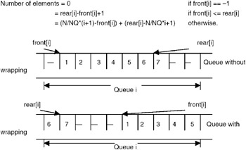
Along with the array nqueue[], front and rear indices for each queue are maintained in arrays front[0…NQ-1] and rear[0…NQ-1].front[i] signifies the first element in queue i. The maximum number of elements in each queue is N/NQ. It is assumed that NQ is a divisor of N. The index of the first element in queue i is given by the formula N/NQ*i.
The program starts by initializing the front and rear of all the queues to a sentinel value (−1). The number of elements in queue i is calculated as follows:
The function qAdd(queue, data) adds data to the end of the queue. It checks for a valid queue number (0…N/NQ-1) and queue-overflow condition. If space is available for the new element in the queue, then rear[queue] is incremented and the new element is inserted at the position. The end condition that the queue was initially empty is also checked as it needs updation of front[queue]. It is possible for rear[queue] to get wrapped to N/NQ*queue.
The function qDelete(queue) removes the front element of the queue. It checks for underflow by using the number of elements in the queue. If the element being deleted is the last element of the queue, rear[queue] is also updated. Otherwise, only front[queue] points to the next element in the queue. It is possible for front[queue] to get wrapped to N/NQ*queue.
The function qIsFul1(queue) checks whether there is any space for a new element. It is implemented by calculating the number of elements in the queue.

Points to Remember

The index of the first element in queue i is calculated as (i* size of each queue).
The complexity of insertion and deletion as described is O(1). Instead, if we do not allow wrapping of elements, then every deletion will cost shifting of elements. That will keep insertion O(1) but deletion would become O(n) where n is the number of elements in the queue.
Since all the queues operate on distinct memory areas, the logic of functions remains the same as in a single queue implementation, except that the calculations are w.r.t. the index of the first element in the queue, compared to an assumed zero for the single queue case.
Note how a single procedure qGetNElements(i), which returns the number of elements in queue i, simplifies corner cases of insertion and deletion, and also simplifies the function qIsFull().

PROBLEM IMPLEMENTATION OF A* ALGORITHM

Given n integers and a sum m,write a program to find the set of integers summing to m by using the A* algorithm.

Program

#include typedef enum {FALSE, TRUE} bool; int subsetsum(int *a, int n, int sum, bool *selected, int startoff) { /* * for those elements a[i] which have selected[i] = FALSE, * solve subsetsum problem for sum. * the elements before startoff are of no use. */ int i: if(sum = 0) return TRUE; for(i=startoff; i0 if e2 is el. * thus we need elements in non-ascending order. */ return *(int *)e2-*(int *)el; } void printAnswer(int *a, int n, bool "selected) { /* * print those a[i] which have selected[i] = TRUE. */ int i; for(i=0; i

Explanation

Inputs are an array a[] of n integers and the sum as another integer. We need to find out a subset of a[] that has the sum of its elements equal to sum. This problem is called a 'subset sum problem.'
The A* algorithm is an A1 technique which chooses the best of the available options to proceed. It uses heuristics that apply to most real-world situations but do not guarantee the best solution. We use the heuristic that courses the element not nearest to the required sum to be added to the current sum.
The list of elements in array a[] is sorted in non-ascending order using the qsort() library function. main() then calls subsetsum(). The function subsetsum() uses the Boolean array selected[n], where selected[i] indicates whether a[i] was included in the sum. The recursive algorithm of subsetsum() follows.
```
boolean subsetsum(a[], n, sum, selected[], startoffset) {
 if(sum == 0)
 return TRUE;
 for i=startoffset to n-1
 if(selected[i] == FALSE && a[i] <= sum) {
 selected[i] = TRUE;
 if(subsetsum(a, n, sum-a[i], selected, i+l) == TRUE)
 return TRUE;
 selected[i] = FALSE;
 }
 return FALSE;
}
```
Thus, if an element has not yet been selected and it is less than the sum, then we choose it and call subsetsum() recursively for the remaining sum by using the elements after this element. The variable startoffset is used to indicate the start of elements which may be of interest to add to the current sum. Since a[i] is selected, no element before a[i+l] will be of interest because all of them are more than a[i], and so are either already selected or greater than the sum. Remember that the elements are in non-increasing order and the sum in different invocations of subsetsum() is also non- increasing. When the sum reaches 0, it indicates the termination condition.
But where in the algorithm have we used the A* algorithm? It is used by first sorting the list in non-increasing order and then traversing it from the highest to the lowest elements. This way, at every step, we choose the option which is nearest to the required sum. If it fails, we deselect the option and choose another option.
Example:
Let a[] = {5,3,4,8,9,6} and sum = 10.
selected[] = {FALSE, FALSE, FALSE, FALSE, FALSE, FALSE}. a[] is sorted to {9,8,6,5,4,3} and subsetsum(a, 6,10, selected, 0) is called. subsetsum() loops over elements 0 to 5 of a.
for i=0, selected[O] = TRUE i.e. a[O] = 9 is selected and subsetsum(a, 6, 10-9, selected, 0+1) is called.
subsetsum() loops over elements 1 to 5 of a.
for i=l, a[l] = 8 > sum 1.
for i=2, a[2] = 6 > sum 1.
…
for i=5, a[5] = 3 > sum 1.
So subsetsum() returns FALSE.
Since subsetsum() returned FALSE, selected[O] = FALSE.
for i=l, selected[l] = TRUE that is, a[l] = 8 is selected and subsetsum(a, 6, 10 -8, selected, 1+1) is called.
subsetsum() returns FALSE in the similar manner as above.
for i=2, selected[2] = TRUE, i.e. a[2] = 6 is selected and subsetsum(a, 6, 10- 6, selected, 2+1) is called.
subsetsum() loops over elements 3 to 5 of a.
for i=3, a[3] = 5 > sum 4.
for i=4, a[4] = 4 <= sum 4.
So selected[4] = TRUE that is a[4] = 4 is selected and subsetsum(a, 6, 4-4, selected, 4+1) is called.
Since sum is 0, subsetsum() returns TRUE.
Since subsetsum() returned TRUE, this subsetsum() returns TRUE.
Since subsetsum() returned TRUE, this subsetsum() returns TRUE to main(). The function printAnswer() then prints the elements a[i] for which selected[i] == TRUE.

Points to Remember

The A* algorithm chooses the best possible of the currently available paths for the next exploration of options.
A* algorithm uses a heuristic. So it does not guarantee the best outcome in all cases. However, in most of the instances of the problem, it is able to reach the solution faster than the algorithm generating all the combinations of the elements.
The complexity of subsetsum() is exponential.
By using the variable startoff, the search space is reduced.

Part I - C Language

Part II - Data Structures

Part III - Advanced Problems in Data Structures