Graphs

Introduction

Graphs are natural models that are used to represent arbitrary relationships among data objects. We often need to represent such arbitrary relationships among the data objects while dealing with problems in computer science, engineering, and many other disciplines. Therefore, the study of graphs as one of the basic data structures is important.

Basic Definitions and Terminology

A graph is a structure made of two components: a set of vertices V, and a set of edges E. Therefore, a graph is G = (V,E), where G is a graph. The graph may be directed or undirected. In a directed graph, every edge of the graph is an ordered pair of vertices connected by the edge, whereas in an undirected graph, every edge is an unordered pair of vertices connected by the edge. Figure 22.1 shows an undirected and a directed graph.

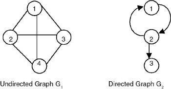
Figure 22.1: Graphs.

Incident edge: (vi,vj) is an edge, then edge(vi,vj) is said to be incident to vertices vi and vj. For example, in graph G1 shown in Figure 22.1, the edges incident on vertex 1 are (1,2), (1,4), and (1,3), whereas in G2, the edges incident on vertex 1 are (1,2).

Degree of vertex: The number of edges incident onto the vertex. For example, in graph G1, the degree of vertex 1 is 3, because 3 edges are incident onto it. For a directed graph, we need to define indegree and outdegree. Indegree of a vertex vi is the number of edges incident onto vi, with vi as the head. Outdegree of vertex vi is the number of edges incident onto vi, with vi as the tail. For graph G2, the indegree of vertex 2 is 1, whereas the outdegree of vertex 2 is 2.

Directed edge: A directed edge between the vertices vi and vj is an ordered pair. It is denoted by .

Undirected edge: An undirected edge between the vertices vi and vj is an unordered pair. It is denoted by (vi,vj).

Path: A path between vertices vp and vq is a sequence of vertices vp, vi1, vi2,…, vin,vq such that there exists a sequence of edges (vp, vi1), (vi1, vi2), …, ( vin, vq). In case of a directed graph, a path between the vertices vp and vq is a sequence of vertices vp, vi1, vi2,…, vin, vq such that there exists a sequence of edges p, vi1>, < vi1, vi2>, …, in, vq>. If there exists a path from vertex vp to vq in an undirected graph, then there always exists a path from vq to vp also. But, in the case of a directed graph, if there exists a path from vertex vp to vq, then it does not necessarily imply that there exists a path from vq to vp also.

Simple path: A simple path is a path given by a sequence of vertices in which all vertices are distinct except the first and the last vertices. If the first and the last vertices are same, the path will be a cycle.

Maximum number of edges: The maximum number of edges in an undirected graph with n vertices is n(n−1)/2. In a directed graph, it is n(n−1).

Subgraph: A subgraph of a graph G = (V,E) is a graph G where V(G) is a subset of V(G). E(G) consists of edges (v1,v2) in E(G), such that both v1 and v2 are in V(G). [Note: If G = (V,E) is a graph, then V(G) is a set of vertices of G and E(G) is a set of edges of G.]

If E(G) consists of all edges (v1,v2) in E(G), such that both v1 and v2 are in V(G), then G is called an induced subgraph of G. For example, the graph shown in Figure 22.2 is a subgraph of the graph G2.

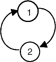
Figure 22.2: The subgraph of graph G2.

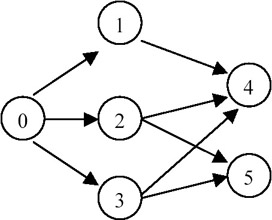
For the graph shown in Figure 22.3, one of the induced subgraphs is shown in Figure 22.4.

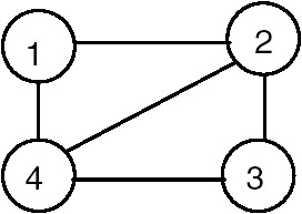
Figure 22.3: Graph G.

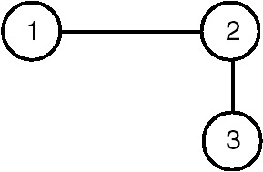
Figure 22.4: Induced subgraph of Graph G of Figure 22.3.

In the undirected graph G, the two vertices v1 and v2 are said to be connected if there exists a path in G from v1 to v2 (being an undirected graph, there exists a path from v2 to v1 also).

Connected graph: A graph G is said to be connected if for every pair of distinct vertices (vi,vj), there is a path from vi to vj. A connected graph is shown in Figure 22.5.

Figure 22.5: A connected graph.

Completely connected graph: A graph G is completely connected if, for every pair of distinct vertices (vi,vj), there exists an edge. A completely connected graph is shown in Figure 22.6.

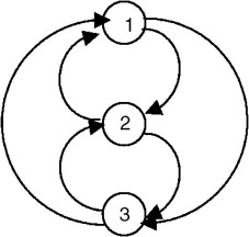
Figure 22.6: A completely connected graph.

REPRESENTATIONS OF A GRAPH

Array Representation

One way of representing a graph with n vertices is to use an n2 matrix (that is, a matrix with n rows and n columns—that means there is a row as well as a column corresponding to every vertex of the graph). If there is an edge from vi to vj then the entry in the matrix with row index as vi and column index as vj is set to 1 (adj[vi, vj] = 1, if (vi, vj) is an edge of graph G). If e is the total number of edges in the graph, then there will 2e entries which will be set to 1, as long as G is an undirected graph. Whereas if G were a directed graph, only e entries would have been set to 1 in the adjacency matrix. The adjacency matrix representation of an undirected as well as a directed graph is show in Figure 22.7.

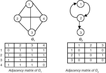
Figure 22.7: Adjacency matrices.

Example

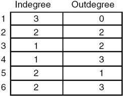
The adjacency matrix representation of the following diagraph(directed graph), along with the indegree and outdegree of each node is shown here:

The adjacency matrix representation of the above diagraph is shown here:

The indegree and outdegree of each node is shown here:

Linked List Representation

Another way of representing a graph G is to maintain a list for every vertex containing all vertices adjacent to that vertex, as shown in Figure 22.8.

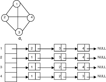
Figure 22.8: Adjacency list of G1.

COMPUTING INDEGREE AND OUTDEGREE OF A NODE OF A GRAPH USING ADJACENCY MATRIX REPRESENTATION

Introduction

To compute the indegree of a node n by using the adjacency matrix representation of a graph, use the node number n as a column index in the adjacency matrix and count the number of 1's in that column of the adjacency matrix. This count is the indegree of node n. Similarly, to compute the outdegree of a node n of a graph, use the node number n as the row index in the adjacency matrix and count the number of 1's in that row of the adjacency matrix. This is the outdegree of the node n. A complete C program to compute the indegree and outdegree of each node of a graph using the adjacency matrix representation of a graph follows.

Program: Computing the indegree and outdegree

#include #define MAX 10 /* a function to build an adjacency matrix of the graph*/ void buildadjm(int adj[][MAX], int n) { int i,j; for(i=0;i

Explanation

1.  
2. This program uses the adjacency matrix representation of a directed graph to compute the indegree and outdegree of each node of the graph.
3.  
4. It first builds an adjacency matrix of the graph by calling a buildadjm function, then goes in a loop to compute the indegree and outdegree of each node by calling the indegree and outdegree functions, respectively.
5.  
6. The indegree function counts the number of 1's in a column of an adjacency matrix using the node number whose indegree is to be computed as a column index.
7.  
8. The outdegree function counts the number of 1's in a row of an adjacency matrix by using the node number whose outdegree is to be computed as a row index.
   •  
   • Input: 1. The number of nodes in a graph 2. Information about edges, in the form of values, to be stored in adjacency matrix 1, if there is an edge from node i to node j; 0 otherwise.
   •  
   • Output: The indegree and outdegree of each node.
   •  
9.  

Example

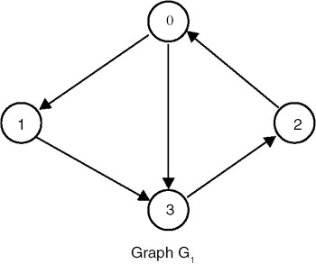
The adjacency matrix for graph G1 is:

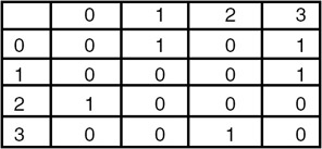
For this graph as the input, the output is:

•  
• The indegree of node 0 is 1
•  
• The outdgree of node 0 is 2
•  
• The indegree of node 1 is 1
•  
• The outdgree of node 1 is 1
•  
• The indegree of node 2 is 1
•  
• The outdgree of node 2 is 1
•  
• The indegree of node 3 is 2
•  
• The outdgree of node 3 is 1
•  

DEPTH FIRST TRAVERSAL

Introduction

A graph can be traversed either by using the depth-first traversal or breadth-first traversal. When a graph is traversed by visiting the nodes in the forward (deeper) direction as long as possible, the traversal is called depth-first traversal. For example, for the graph shown in Figure 22.9, the depth-first traversal starting at the vertex 0 visits the node in the orders:

1.  
2. 0 1 2 6 7 8 5 3 4
3.  
4. 0 4 3 5 8 6 7 2 1
5.  

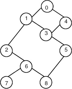Figure 22.9: Graph G and its depth first traversals starting at vertex 0.

A complete C program for depth-first traversal of a graph follows. It makes use of an array visited of n elements where n is the number of vertices of the graph, and the elements are Boolean. If visited[i] = 1 then it means that the ith vertex is visited. Initially we set visited[i] = 0.

Program

#include #define max 10 /* a function to build adjacency matrix of a graph */ void buildadjm(int adj[][max], int n) { int i,j; for(i=0;i

Explanation

1.  
2. Initially, all the elements of an array named visited are set to 0 to indicate that all the vertices are unvisited.
3.  
4. The traversal starts with the first vertex (that is, vertex 0), and marks it visited by setting visited[0] to 1. It then considers one of the unvisited vertices adjacent to it and marks it visited, then repeats the process by considering one of its unvisited adjacent vertices.
5.  
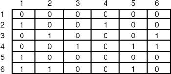
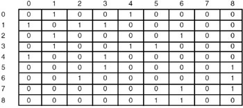
6. Therefore, if the following adjacency matrix that represents the graph of Figure 22.9 is given as input, the order in which the nodes are visited is given here:
   •  
   • Input: 1. The number of nodes in a graph 2. Information about edges, in the form of values to be stored in adjacency matrix 1 if there is an edge from node i to node j, 0 otherwise
   •  
   • Output: Depth-first ordering of the nodes of the graph starting from the initial vertex, which is vertex 0, in our case.
   •  
7.  

Example

Input

Output

0, 1, 2, 6, 8, 5, 3, 4, 7

Analysis

1.  
2. If the graph G to which the depth-first search (dfs) is applied is represented using adjacency lists, then the vertices y adjacent to x can be determined by following the list of adjacent vertices for each vertex.
3.  
4. Therefore, the for loop searching for adjacent vertices has the total cost of d1 + d2 +…+ dn, where di is the degree of vertex vi, because the number of nodes in the adjacency list of vertex vi are di.
5.  
6. If the graph G has n vertices and e edges, then the sum of the degree of each vertex (d1 + d2 + …+ dn) is 2e. Therefore, there are total of 2e list nodes in the adjacency lists of G. If G is a directed graph, then there are a total of e list nodes only.
7.  
8. The algorithm examines each node in the adjacency lists once, at most. So the time required to complete the search is O(e), provided n<= e. Instead of using adjacency lists, if an adjacency matrix is used to represent a graph G, then the time required to determine all adjacent vertices of a vertex is O(n), and since at most n vertices are visited, the total time required is O(n2).
9.  

BREADTH FIRST TRAVERSAL

Introduction

When a graph is traversed by visiting all the adjacent nodes/vertices of a node/vertex first, the traversal is called breadth-first traversal. For example, for a graph in which the breadth-first traversal starts at vertex v1, visits to the nodes take place in the order shown in Figure 22.10.

Figure 22.10: Breadth-first traversal of graph G starting at vertex v1.

Program

A complete C program for breadth-first traversal of a graph appears next. The program makes use of an array of n visited elements where n is the number of vertices of the graph. If visited[i] = 1, it means that the ith vertex is visited. The program also makes use of a queue and the procedures addqueue and deletequeue for adding a vertex to the queue and for deleting the vertex from the queue, respectively. Initially, we set visited[i] = 0.

#include #include #define MAX 10 struct node { int data; struct node *link; }; void buildadjm(int adj[][MAX], int n) { int i,j; printf("enter adjacency matrix ",i,j); for(i=0;idata = val; p->link=NULL; } else { temp= p; while(temp->link != NULL) { temp = temp->link; } temp->link = (struct node*)malloc(sizeof(struct node)); temp = temp->link; if(temp == NULL) { printf("Cannot allocate "); exit(0); } temp->data = val; temp->link = NULL; } return(p); } struct node *deleteq(struct node *p,int *val) { struct node *temp; if(p == NULL) { printf("queue is empty "); return(NULL); } *val = p->data; temp = p; p = p->link; free(temp); return(p); } void bfs(int adj[][MAX], int x,int visited[], int n, struct node **p) { int y,j,k; *p = addqueue(*p,x); do{ *p = deleteq(*p,&y); if(visited[y] == 0) { printf(" node visited = %d ",y); visited[y] = 1; for(j=0;j

Example

Input and Output

Enter the number of nodes in graph maximum = 10 9

Enter adjacency matrix

0 1 0 0 1 0 0 0 0
1 0 1 1 0 0 0 0 0
0 1 0 0 0 0 1 0 0
0 1 0 0 1 1 0 0 0
1 0 0 1 0 0 0 0 0
0 0 0 1 0 0 0 0 1
0 0 1 0 0 0 0 1 1
0 0 0 0 0 0 1 0 0
0 0 0 0 0 1 1 0 0
node visited = 0
node visited = 1
node visited = 4
node visited = 2
node visited = 3
node visited = 6
node visited = 5
node visited = 7
node visited = 8

 

 

CONNECTED COMPONENT OF A GRAPH

Introduction

The connected component of a graph is a maximal subgraph of a given graph, which is connected. For example, consider the graph that follows.

The connected component of the graph G1 is shown in Figure 22.11.

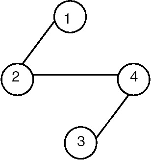
Figure 22.11: Connected component of G1.

Strongly Connected Component

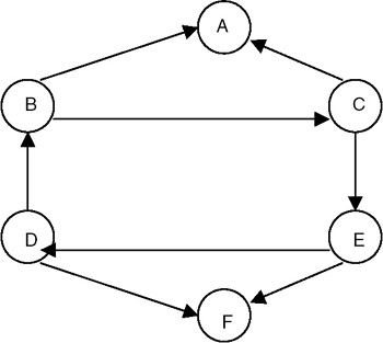
For a diagraph (directed graph), a strongly connected component is that component of the graph in which, for every pair of distinct vertices vi and vj, there is a directed path from vi to vj, and also a directed path from vj to vi. For example, consider the diagraph shown in Figure 22.12.

Figure 22.12: A diagraph.

The strongly connected components of the graph are shown in Figure 22.13.

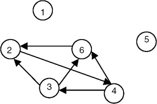
Figure 22.13: Strongly connected components of the graph shown in Figure 22.12.

Example

Is the following diagraph strongly connected?

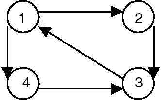
This table shows the possible pairs of vertices, and the forward and backward paths between them, for the previous graph:

PAIR OF VERTICES	FORWARD PATH	BACKWARD PATH
<1, 2>	1-2	2-3-4
<1,3>	1-2-3	3-1
<1,4>	1-4	4-3-1
<2,3>	2-3	3-1-2
<2,4>	2-3-1-4	4-3-1-2
<3,4>	3-1-4	4-3

Therefore, we see that between every pair of distinct vertices of the given graph there exists a forward as well as a backward path, so it is strongly connected.

Program

Write a function dfs(v) to traverse a graph in a depth-first manner starting from vertex v. Use this function to find connected components in the graph. Modify dfs() to produce a list of newly visited vertices. The graph is represented as adjacency lists.

#include #define MAXVERTICES 20 #define MAXEDGES 20 typedef enum {FALSE, TRUE, TRISTATE} bool; typedef struct node node; struct node { int dst; node *next; }; void printGraph( node *graph[], int nvert ) { /* * prints the graph. */ int i, j; for( i=0; inext ) printf( "[%d] ", ptr->dst ); printf( " " ); } } void insertEdge( node **ptr, int dst ) { /* * insert a new node at the start. */ node *newnode = (node *)malloc( sizeof(node) ); newnode->dst = dst; newnode->next = *ptr; *ptr = newnode; } void buildGraph( node *graph[], int edges[2][MAXEDGES], int nedges ) { /* * fills graph as adjacency list from array edges. */ int i; for( i=0; inext ) if( visited[ ptr->dst ] == FALSE ) dfs( ptr->dst, visited, graph ); } void printSetTristate( int *visited, int nvert ) { /* * prints all vertices of visited which are TRISTATE. * and set them to TRUE. */ int i; for( i=0; i

Explanation

1.  
2. The graph is represented as adjacency lists. The graph contains an array of n pointers where n is the number of vertices in the graph. Each entry i in the array contains a list of vertices to which i is connected. For example, if the graph is as shown in the first diagram, the adjacency lists for the graph are as shown in the subsequent diagram.

   

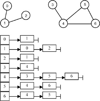
   Each node in list i contains a vertex to which i is connected.

3.  
4. dfs(v) is implemented recursively. A Boolean vector visited[] is maintained whose entries are initially all FALSE. dfs(v) marks v as visited by making visited[v] = TRUE. It then finds all the adjacent nodes of v and starts dfs() from those nodes that have not yet been visited. For example, if dfs(v) is called with v == 0, it marks 0 and then it traverses the adjacency list graph[0] and calls dfs(1). This marks 1 and traverses the adjacency list graph[1]. But since 0 is already marked, dfs(2) is called. It marks 2 and starts traversal of graph[2]. But since 1 is marked, it returns. All the previous invocations return as there are no nodes being considered in the lists. Thus, the marked vertices are {0, 1, 2}.
5.  
6. compINC() is a function that finds all the connected components of a graph. It maintains a local copy of the vector visited[] and passes it as a parameter to dfs(v). compINC() passes that vertex as a parameter to dfs() that has not yet been visited. Thus each invocation of dfs() finds one connected component of the graph.
7.  
8. In order to modify dfs() to produce a list of newly visited vertices, we tag the vertices visited using dfs() as TRISTATE. In compINC(), all these TRISTATE vertices will form one connected component. This status is then converted to TRUE. The next invocation to dfs() returns another set of vertices tagged as TRISTATE, which forms another connected component and so on.
9.  

For example, in the previous program, first all vertices are tagged as FALSE. After the invocation of dfs(0), the vertices tagged as TRISTATE are {0, 1, 2}. These are output and their tags are changed from TRISTATE to TRUE. The next invocation of dfs(3) tags vertices {3, 4, 5, 6} as TRISTATE. These are then output and their tags are changed from TRISTATE to TRUE. Since there is no vertex remaining whose tag is FALSE, the algorithm stops.

Points to Remember

1.  
2. All the reachable vertices can be traversed from a source vertex by using depth-first search.
3.  
4. The data representation (a graph in this case) should be such that it should make algorithms operate on the data efficiently. Being represented as adjacency lists, we could easily traverse the list to get the vertices adjacent to a particular vertex.
5.  
6. Note how a simple recursive procedure solves the problem of finding all the reachable vertices from a vertex.
7.  
8. Note the use of descriptive words such as FALSE, TRUE and TRISTATE, rather than integers 0, 1 and 2. It makes the program easily understandable.
9.  

DEPTH FIRST SPANNING TREE AND BREADTH FIRST SPANNING TREE

Introduction

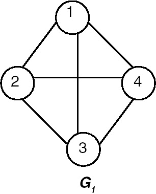
If graph G is connected, the edges of G can be partitioned into two disjointed sets. One is a set of tree edges, which we denote by set T, and the other is a set of back edges, which we denote by B. The tree edges are precisely those edges that are followed during the depth-first traversal or during the breadth-first traversal of graph G. If we consider only the tree edges, we get a subgraph of G containing all the vertices of G, and this subgraph is a tree called spanning tree of the graph G. For example, consider the graph shown in Figure 22.14.

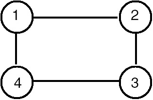Figure 22.14: Graph G.

One of the depth-first traversal orders for this tree is 1-2-3-4, so the tree edges are (1,2), (2,3) and (3,4). Therefore, one of the spanning trees obtained by using depth-first traversal of the graph of Figure 22.14 is shown in Figure 22.15.

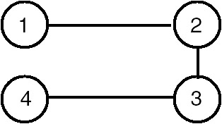Figure 22.15: Depth first spanning tree of the graph of Figure 22.14.

Similarly, one of the breadth-first traversal orders for this tree is 1-2-4-3, so the tree edges are (1,2), (1,4) and (4,3). Therefore, one of the spanning trees obtained using breadth-first traversal of the graph of Figure 22.14 is shown in Figure 22.16.

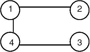Figure 22.16: Breadth-first spanning tree of the graph of Figure 22.14.

The algorithm for obtaining the depth-first spanning tree (dfst) appears next.

T = f; {initially set of tree nodes is empty}
dfst( v : node);
{
 if (visited[v] = false)
 {
 visited[v] = true;
 for every adjacent i of v do
 {
 T = T È {(v,i)}
 dfst(i);
 }
 }
}

If a graph G is not connected, the tree edges, which are precisely those edges followed during the depth-first, traversal of the graph G, constitute the depth-first spanning forest. The depth-first spanning forest will be made of trees, each of which is one of the connected components of graph G.

When a graph G is directed, the tree edges, which are precisely those edges followed during the depth-first traversal of the graph G, form a depth-first spanning forest for G. In addition to this, there are three other types of edges. These are called back edges, forward edges, and cross edges. An edge A →B is called a back edge, if B is an ancestor of A in the spanning forest. A non-tree edge that goes from a vertex to a proper descendant is called a forward edge. An edge which goes from a vertex to another vertex that is neither an ancestor nor a descendant is called a cross edge. An edge from a vertex to itself is a back edge. For example, consider the directed graph G shown in Figure 22.17.

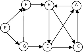
Figure 22.17: A directed graph G.

The depth-first spanning forest for graph G of Figure 22.17 is shown in Figure 22.18.

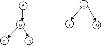
Figure 22.18: Depth-first spanning forest for the graph G of Figure 22.17.

In graph G of Figure 22.17, the edges such as C → A and D → A are the back edges, the edges such as D → C and G → D are cross edges.

Example

Consider the graph shown in Figure 22.19.

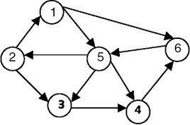
Figure 22.19: A graph G.

If we apply the procedure dfst to this graph, one of the depth-first spanning trees that we get by starting with vertex 1 is shown in Figure 22.20.

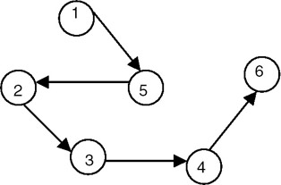
Figure 22.20: Depth-first spanning tree of the graph G of Figure 22.19.

 

 

MINIMUM COST SPANNING TREE

Introduction

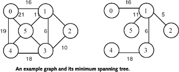
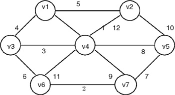
When the edges of the graph have weights representing the cost in some suitable terms, we can obtain that spanning tree of a graph whose cost is minimum in terms of the weights of the edges. For this, we start with the edge with the minimum-cost/weight, add it to set T, and mark it as visited. We next consider the edge with minimum-cost that is not yet visited, add it to T, and mark it as visited. While adding an edge to the set T, we first check whether both the vertices of the edge are visited; if they are, we do not add to the set T, because it will form a cycle. For example, consider the graph shown in Figure 22.21.

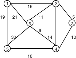
Figure 22.21: A graph G.

The minimum-cost spanning tree of the graph of Figure 22.21 is shown in Figure 22.22.

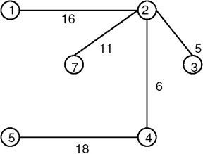
Figure 22.22: The minimum-cost spanning tree of graph G of Figure 22.21.

MST Property

Let G = (V,E) be a connected graph with a cost function defined on the edges. Let U be some proper subset of the set of vertices V. If (u,v) is an edge of lowest cost such that u is in U, and v is in V-U, there is a minimum-cost spanning tree that includes edge (u,v). Many of the methods of constructing a minimum-cost spanning tree use the following properties.

Prim's Algorithm

Let G = (V,E) be a weighted graph, and suppose V = {1,2,…,n}. The Prim's algorithm begins with a set U initialized to {1}, and at each stage finds the shortest edge (u,v) that connects u in U and v in V-U, and then adds v to U. It repeats this step until U = V.

mcost(G is a graph; T is a set of edges)
 U is a set of vertices
 u,v are vertices;
{
 T= ô
 U = {1}
 while U '" V
 {

Find the lowest-cost edge (u,v) such that u is in U and v is in V-U

 add (u,v) to T
 add v to U
 }
}

Program

The following program can be used to find the minimum spanning tree of a graph.

#include #define MAXVERTICES 10 #define MAXEDGES 20 typedef enum {FALSE, TRUE} bool; int getNVert(int edges[][3], int nedges) { /* * returns no of vertices = maxvertex + 1; */ int nvert = −1; int j; for( j=0; j nvert ) nvert = edges[j][0]; if( edges[j][1] > nvert ) nvert = edges[j][1]; } return ++nvert; // no of vertices = maxvertex + 1; } bool isPresent(int edges[][3], int nedges, int v) { /* * checks whether v has been included in the spanning tree. * thus we see whether there is an edge incident on v which has * a negative cost. negative cost signifies that the edge has been * included in the spanning tree. */ int j; for(j=0; j−1; ++i) for(j=i; j edges[j][2]) { tv1 = edges[i][0]; tv2 = edges[i][1]; tcost = edges[i][2]; edges[i][0] = edges[j][0]; edges[i][1] = edges[j][1]; edges[i][2] = edges[j][2]; edges[j][0] = tv1; edges[j][1] = tv2; edges[j][2] = tcost; } for(j=0; j

Explanation

1.  
2. A tree consisting solely of edges in a graph G, and including all vertices in G, is called a spanning tree. A minimum spanning tree of a weighted graph is the spanning tree with minimum total cost of its edges.

   

3.  
4. The graph is represented as an array of edges. Each entry in the array is a triplet representing an edge consisting of source vertex, destination vertex, and the cost associated with the edge. The method used in finding a minimum spanning tree is that given by Kruskal. In this approach, a minimum spanning tree T is built edge by edge. Edges are considered for inclusion in T in non- decreasing order of their costs. An edge is included if it does not form a cycle with the edges that are already in T. Since graph G is connected and has n > 0 vertices, exactly n − 1 edges will be selected for inclusion in T.
5.  
6. Kruskal's algorithm is as follows:

   T={}; // empty set.
   while T contains less than n-1 edges and E not empty do
    choose an edge (v, w) from E of lowest cost.
    delete (v, w) from E.
    if (v, w) does NOT create a cycle in T
    add (v, w) to T.
    else
    discard (v, w).
   endwhile.
   if T contains less than n-1 edges
    print("no spanning tree exists for this graph.");
   

7. In order for the choice of the lowest-cost edge from E to become efficient, we sort the edge array over the cost of edge. To check whether an edge (v, w) forms a cycle, we simply need to check whether both v and w appear in any of the previously added edges in T. We assume that all the costs are positive and we make them negative to signify that the edge has been included in T.
8. Example:

   For the example graph in item 1, the run of the algorithm goes as follows:

   STEP	EDGE	COST	ACTION	SPANNING-TREE
   0	—	—	—	{}.
   1	(1, 2)	5	accept	{(1, 2)}.
   2	(1, 3)	6	accept	{(1, 2), (1, 3)}.
   3	(2, 3)	10	reject	{(1, 2), (1, 3)}.
   4	(1, 5)	11	accept	{(1, 2), (1, 3), (1, 5)}.
   5	(3, 5)	14	reject	{(1, 2), (1, 3), (1, 5)}.
   6	(0, 1)	16	accept	{(1, 2), (1, 3), (1, 5), (0, 1)}.
   7	(3, 4)	18	accept	{(1, 2), (1, 3), (1, 5), (0, 1), (3, 4)}.

Points to Remember

1. A minimum spanning tree of a weighted graph G is a tree that consists of edges solely from the edges of G, which covers all the vertices in G, and which has the minimum combined cost of its edges.
2. The complexity of Kruskal's method used for finding the minimum spanning tree of a graph G is O(eloge) where e is the number of edges in G.
3. Note that the union and find algorithms for set representation can be used for checking for cycle and inclusion of an edge in a set.
4. There can be multiple minimum spanning trees in a graph.

Application of Minimum Cost Spanning Tree

A property of a spanning tree of a graph G is that a spanning tree is a minimal connected subgraph of G (by minimal, we mean the one with the fewest number of edges). Therefore, if nodes of G represent cities and the edges represent possible communication links connecting two cities, then the spanning trees of graph G represent all feasible choices of the communication network. If each edge has weight representing cost measured in some suitable terms (such as cost of construction or distance etc.), then the minimum-cost spanning tree of G is the selection of the required communication network.

 

 

DIRECTED ACYCLIC GRAPH (DAG)

Concept

A directed acyclic graph (DAG) is a directed graph with no cycles. A DAG represents more general relationships than trees but less general than arbitrary directed graphs. An example of a DAG is given in Figure 22.23.

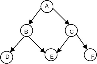
Figure 22.23: Directed acyclic graph.

DAGs are useful in representing the syntactic structure of arithmetic expressions with common sub-expressions. For example, consider the following expression:

(a+b)*c + ((a+b + e)

In this expression, the term (a + b) is a common sub-expression, and therefore represented in the DAG by the vertices with more than one incoming edge, as shown in Figure 22.24.

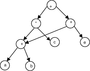
Figure 22.24: DAG representation of expression (a+b)*c +((a+b) + e).

Topological Sort of Directed Graph

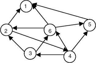
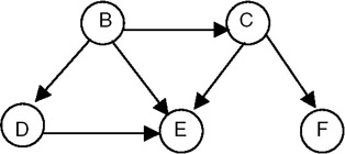
A topological sort is a method for ordering the nodes of the directed graph G in which the nodes represent tasks or activities, and the edges represent precedence relations between nodes, that is, when the edges of the graph represent dependency among the node/vertices of graph G. It lists the vertices/nodes in such an order that a vertex vi gets listed only after all the vertices on which vi depends have been listed. For a topological sort to be feasible, it is required that the directed graph G not have any directed cycles. In other words, the graph G should be a DAG. This also means that the precedence relation defined by the edges of G must be irreflexive. The precedence relation defined by the edges of G is certainly transitive and so is a partial order. It starts with a vertex that does not have any predecessor and lists it. After that it logically deletes it from the graph and once again searches for that vertex that does not have any predecessor, and repeats the procedure. It does not give a unique order. For example, consider the directed graph shown in Figure 22.25.

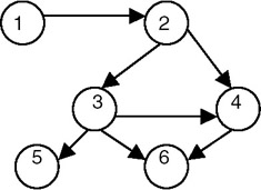
Figure 22.25: A graph G.

The topological sort of the graph in Figure 22.25 gives the following orders:

• 1-2-3-4-5-6
• 1-2-3-5-4-6
• 1-2-3-4-6-5

The algorithm for a topological sort is presented here:

while there exist a node
 {
 select a node which does not have any predecessor
 list the selected node
 delete it from the graph
 }

The procedure for a depth first search, with a print statement added to print the nodes, can also be used, as shown in the following program, to perform a topological sort. This algorithm prints the vertices accessible from x in reverse topological sort. This algorithm prints the vertices accessible from x in reverse topological order.

Program

Write a program to find the topological order of a diagraph G represented as adjacency lists.

#include 

#define N 11 // no of total vertices in the graph.

typedef enum {FALSE, TRUE} bool;
typedef struct node node;

struct node {
 int count; // for arraynodes : in-degree.
 // for listnodes : vertex no this vertex is connected to.
 // if this node is out of graph : −1.
 // if this has 0 indegree then it occurs in zerolist.
 node *next;
};

node graph[N];
node *zerolist;

void addToZerolist( int v ) {
 /*
 * adds v to zerolist as v has 0 predecessors.
 */
 node *ptr = (node *)malloc( sizeof(node) );
 ptr->count = v;
 ptr->next = zerolist;
 zerolist = ptr;
}

void buildGraph( int a[][2], int edges ) {
 /*
 * fills global graph with input given in a.
 * a[i][0] is src vertex and a[i][1] is dst vertex.
 */
 int i;

 // init graph.
 for( i=0; icount = a[i][1];
 ptr->next = graph[ a[i][0] ].next;
 graph[ a[i][0] ].next = ptr;
 // increase indegree of dst.
 graph[ a[i][1] ].count++;
 }

 // now create list of zero predecessors.
 zerolist = NULL; // list of vertices having 0 predecessors.
 for( i=0; inext )
 printf( "%d ", ptr->count );
 printf( "
" );
 }
 printf( "zerolist: " );
 for( ptr=zerolist; ptr; ptr=ptr->next )
 printf( "%d ", ptr->count );
 printf( "
" );
 }

 int getZeroVertex() {
 /*
 * returns the vertex with zero predecessors.
 * if no such vertex then returns −1.
 */
 int v;
 node *ptr;

 if( zerolist == NULL )
 return −1;
 ptr = zerolist;
 v = ptr->count;
 zerolist = zerolist->next;
 free(ptr);

 return v;
 }

 void removeVertex( int v ) {
 /*
 * deletes vertex v and its outgoing edges from global graph.
 */
 node *ptr;
 graph[v].count = −1;
 // free the list graph[v].next.
 for( ptr=graph[v].next; ptr; ptr=ptr->next ) {
 if( graph[ ptr->count ].count > 0 ) // normal nodes.
 graph[ ptr->count ].count-;
 if( graph[ ptr->count ].count == 0 ) // this is NOT else of above if.
 addToZerolist( ptr->count );
 }
}

void topsort( int nvert ) {
 /*
 * finds recursively topological order of global graph.
 * nvert vertices of graph are needed to be ordered.
 */
 int v;

 if( nvert > 0 ) {
 v = getZeroVertex();
 if( v == −1 ) { // no such vertex.
 fprintf( stderr, "graph contains a cycle.
" );
 return;
 }
 printf( "%d.
", v );
 removeVertex(v);
 topsort( nvert-1 );
 }
}

int main() {
 int a[][2] = {
 {0,1},
 {0,3},
 {0,2},
 {1,4},
 {2,4},
 {2,5},
 {3,4},
 {3,5}
 };
 buildGraph( a, 8 );
 printGraph();
 topsort(N);
}

Explanation

1. A linear ordering of vertices of a diagraph G, with the property that if i is a predecessor of j then i precedes j in linear order, is called a topological order of G.
2. The diagraph G is maintained as adjacency lists. In this representation, G is an array graph[0..n-1] where each element graph[i] is a linked list of vertices. Vertex i is connected to, and n is the number of, vertices in G.
3. We also maintain a zerolist, which is a list of vertices that have zero predecessors. The necessity of this list will be clear in the algorithm shown in number four of this explanation.
4. The algorithm for topological sort is:

   topsort(n) {
    if( n > 0 ) {
   if every vertex has a predecessor then
    error( "graph contains a cycle." ).
   pick a vertex v that has no predecessors. // getZeroVertex()
   output v.
   delete v and all the edges leading out of v in the graph. // removeVertex()
   topsort(n-1).
    }
   }
   

5. The algorithm topsort() is tail-recursive. From zerolist, it removes a vertex v containing zero predecessors and outputs it. This vertex v has no predecessors in G or all its predecessors have already been output. Thus all the vertices in zerolist are the candidates for the next output. After v is output, all the vertices to which v points may become the candidates for the next output. Thus we remove all the edges starting from v and rerun topsort() over the remaining vertices.
6. See the following example of a diagraph.

   

STEP	ZEROLIST	OUTPUT
0	{0}	nil
1	{1, 2, 3}	0
2	{2, 3}	1
3	{3}	2
4	{4,5}	3
5	{5}	4
6	{}	5

Points to Remember

1. A linear ordering of vertices of a diagraph G, with the property that if i is a predecessor of j then i precedes j in the linear ordering, is called a topological order of G.
2. The complexity of topological order is O(n+e) where n is the number of vertices and e is the number of edges in the diagraph.
3. Removal of an edge results in a decrease in the predecessor count of the destination vertex. If this count reaches 0, the vertex should be inserted in the zerolist.
4. By maintaining a list of vertices with zero predecessors, the computing time of the algorithm decreases.
5. The algorithm is therefore a total time of O(e), if graph G is represented by an adjacency list, and O(n2) if graph G is represented by an adjacency matrix.

General Comments on Graphs

1. A graph is a structure that is often used to model the arbitrary relationships among the data objects while solving many problems.
2. A graph is a structure made of two components: a set of vertices V, and the set of edges E. Therefore, a graph is G = (V,E), where G is a graph.
3. The graph may be directed or undirected. When the graph is directed, every edge of the graph is an ordered pair of vertices connected by the edge.
4. When the graph is undirected, every edge of the graph is an unordered pair of vertices connected by the edge.
5. The maximum number of edges in an undirected graph with n vertices is n(n − 1)/2, whereas in the case of a directed graph, it is n(n − 1).
6. Adjacency matrices and adjacency lists are used to represent graphs.
7. A graph can be traversed by using either the depth first traversal or the breadth first traversal.
8. When a graph is traversed by visiting in the forward (deeper) direction as long as possible, the traversal is called depth first traversal.
9. When a graph is traversed by visiting all the adjacencies of a node/vertex first, the traversal is called breadth first traversal.
10. A connected component of a graph is a maximal subgraph of a given graph that is connected.
11. A DAG is an important data structure used for representing syntactic structure of expressions with common subexpressions.
12. A DAG is also used in representing partial orders.
13. A topological sort lists the vertices in such an order that if a vertex vi is a predecessor of vertex vj then vi precedes vj in the linear ordering.
14. Topological sort is possible only for a DAG.

Exercises

1. Find out the minimum number of edges in a strongly connected diagraph on n vertices.
2. Test the program for obtaining the depth first spanning tree for the following graph:

   

3. Test the program for obtaining the minimum cost spanning tree for the following graph:

   

4. Test a program for topological sort for the following DAG: