Arrays, Searching, and Sorting

ARRAYS

Introduction

An array is a fixed-sized, homogeneous, and widely-used data structure. By homogeneous, we mean that it consists of components which are all of the same type, called element type or base type. And by fixed sized, we mean that the number of components is constant, and so does not change during the lifetime of the structure. An array is also called a random-access data structure, because all components can be selected at random and are equally accessible. An array can be used to structure several data objects in the programming languages. A component of an array is selected by giving its subscript, which is an integer indicating the position of the component in the sequence. Therefore, an array is made of the pairs (value, index); it means that with every index, a value is associated. If every index is one single value then it is called a one-dimensional array, whereas if every index is a n-tuple {i1, i2, i3,….., in}, the array is called a n-dimensional array.

Memory Representation

An array is represented in memory by using a sequential mapping. The basic characteristic of the sequential mapping is that every element is at a fixed distance apart. Therefore, if the ith element is mapped into a location having an address a, then the (i + 1)th element is mapped into the memory location having an address (a + 1), as shown in Figure 18.1.

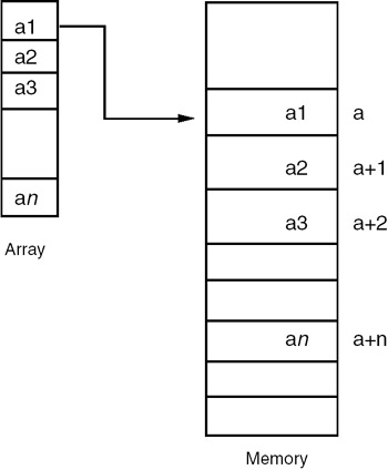
Figure 18.1: Representation of an array.

The address of the first element of an array is called the base address, so the address of the the ith element is

Base address + offset of the ith element from base address

where the offset is computed as:

Offset of the ith element = number of elements before the ith *

size of each element.

If LB is the lower bound, then the offset computation becomes:

offset = (i − LB) * size.

Representation of Two-Dimensional Array

A two-dimensional array can be considered as a one-dimensional array whose elements are also one-dimensional arrays. So, we can view a two dimensional array as one single column of rows and map it sequentially as shown in Figure 18.2. Such a representation is called a row-major representation.

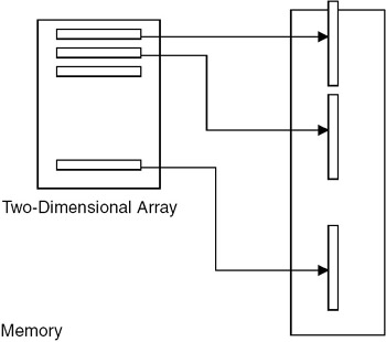
Figure 18.2: Row-major representation of a two-dimensional array.

The address of the element of the ith row and the jth column therefore is:

addr(a[i, j]) = ( number of rows placed before ith row * size of a row) + (number of elements placed before the jth element in the ith row * size of element)

where

Number of rows placed before ith row = (i – LB1), and LB1 is the lower bound of the first dimension.

Size of a row = number of elements in a row * a size of element.

Number of elements in a row = (UB2 – LB2+1), where UB2 and LB2 are the upper and lower bounds of the second dimension, respectively.

Therefore:

addr(a[i, j]) = ((i − LB1) * (UB2 − LB2+1) * size) + ((j − LB2)*size)

It is also possible to view a two-dimensional array as one single row of columns and map it sequentially as shown in Figure 18.3. Such a representation is called a column-major representation.

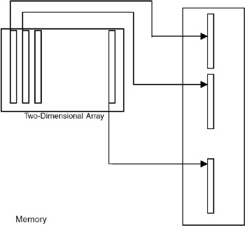
Figure 18.3: Column major representation of a two-dimensional array.

The address of the element of the ith row and the jth column therefore is:

addr(a[i, j]) = ( number of columns placed before jth column * size of a column) + (number of elements placed before the ith element in the jth column * size of each element)

Number of columns placed before jth column = (j − LB2) where LB2 is the lower bound of the second dimension.

Size of a column = number of elements in a column * size of element Number of elements in a column = (UB1 – LB1 + 1), where UB1 and LB1 are the upper and lower bounds of the first dimension, respectively.

Therefore:

addr(a[i, j]) = ((j − LB2) * (UB1 − LB1+1) * size) + ((i − LB1)*size)

APPLICATION OF ARRAYS

Whenever we require a collection of data objects of the same type and want to process them as a single unit, an array can be used, provided the number of data items is constant or fixed. Arrays have a wide range of applications ranging from business data processing to scientific calculations to industrial projects.

Implementation of a Static Contiguous List

A list is a structure in which insertions, deletions, and retrieval may occur at any position in the list. Therefore, when the list is static, it can be implemented by using an array. When a list is implemented or realized by using an array, it is a contiguous list. By contiguous, we mean that the elements are placed consecutively one after another starting from some address, called the base address. The advantage of a list implemented using an array is that it is randomly accessible. The disadvantage of such a list is that insertions and deletions require moving of the entries, and so it is costlier. A static list can be implemented using an array by mapping the ith element of the list into the ith entry of the array, as shown in Figure 18.4.

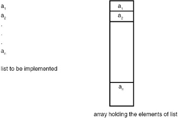
Figure 18.4: Implementation of a static contiguous list.

Program

A complete C program for implementing a list with operations for reading values of the elements of the list and displaying them is given here:

#include #include void main() { void read(int *,int); void dis(int *,int); int a[5],i,sum=0; clrscr(); printf("Enter the elements of array "); read(a,5); /*read the array*/ printf("The array elements are "); dis(a,5); } void read(int c[],int i) { int j; for(j=0;j

Example

Input

Enter the elements of the first array

15
30
45
60
75

Output

The elements of the first array are

15 30 45 60 75

 

 

MANIPULATIONS ON THE LIST IMPLEMENTED USING AN ARRAY

Introduction

Shown next are C programs for carrying out manipulations such as finding the sum of elements of an array, adding two arrays, and reversing an array.

Program

ADDITION OF THE ELEMENTS OF THE LIST #include #include void main() { void read(int *,int); void dis(int *,int); int a[5],i,sum=0; clrscr(); printf("Enter the elements of list "); read(a,5); /*read the list*/ printf("The list elements are "); dis(a,5); for(i=0;i<5;i++) { sum+=a[i]; } printf("The sum of the elements of the list is %d ",sum); getch(); } void read(int c[],int i) { int j; for(j=0;j

Example

Input

Enter the elements of the first array

15
30
45
60
75

Output

The elements of the first array are

15 30 45 60 75

The sum of the elements of an array is 225.

Addition of the two lists

Suppose the first list is

1
2
3
4
5

and the second list is

5
6
8
9
10

The first element of first list is added to the first element of the second list, and the result of the addition is the first element of the third list.

In this example, 5 is added to 1, and the first element of third list is 6.

This step is repeated for all the elements of the lists and the resultant list after the addition is

6
8
11
13
15

#include #include void main() { void read(int *,int); void dis(int *,int); void add(int *,int *,int * ,int); int a[5],b[5],c[5],i; clrscr(); printf("Enter the elements of first list "); read(a,5); /*read the first list*/ printf("The elements of first list are "); dis(a,5); /*Display the first list*/ printf("Enter the elements of second list "); read(b,5); /*read the second list*/ printf("The elements of second list are "); dis(b,5); /*Display the second list*/ add(a,b,c,i); printf("The resultant list is "); dis(c,5); getch(); } void add(int a[],int b[],int c[],int i) { for(i=0;i<5;i++) { c[i]=a[i]+b[i]; } } void read(int c[],int i) { int j; for(j=0;j

Explanation

1.  
2. Repeat step (2) for i=0,1,2,… (n−1), where n is the maximum number of elements in a list.
3.  
4. c[i] = a[i]+b[i], where a is the first list, b is the second list, and c is the resultant list; a[i] denotes the ith element of list a.
5.  

Example

Input

Enter the elements of the first list

1
2
3
4
5

Output

The elements of the first list are

2 3 4 5

Input

Enter the elements of the second list

6
7
8
9
10

Output

The elements of the second list are

6 7 8 9 10

The resultant list is

7 9 11 13 15

Inverse of the list

The following program makes a reverse version of the list.

#include #include void main() { void read(int *,int); void dis(int *,int); void inverse(int *,int); int a[5],i; clrscr(); read(a,5); dis(a,5); inverse(a,5); dis(a,5); getch(); } void read(int c[],int i) { int j; printf("Enter the list "); for(j=0;j

Example

Input

Enter the list

10
20
30
40
50

Output

The list is

10 20 30 40 50

The inverse of the list is

50 40 30 20 10

This is another version of an inverse program, in which another list is used to hold the reversed list.

#include #include void main() { void read(int *,int); void dis(int *,int); void inverse(int *,int *,int); int a[5],b[5]; clrscr(); read(a,5); dis(a,5); inverse(a,b,5); dis(b,5); getch(); } void read(int c[],int i) { int j; printf("Enter the list "); for(j=0;j

Example

Input

Enter the list

10
20
30
40
50

Output

The list is

10 20 30 40 50

The inverse of the list is

50 40 30 20 10

 

 

MERGING OF TWO SORTED LISTS

Introduction

Assume that two lists to be merged are sorted in descending order. Compare the first element of the first list with the first element of the second list. If the element of the first list is greater, then place it in the resultant list. Advance the index of the first list and the index of the resultant list so that they will point to the next term. If the element of the first list is smaller, place the element of the second list in the resultant list. Advance the index of the second list and the index of the resultant list so that they will point to the next term.

Repeat this process until all the elements of either the first list or the second list are compared. If some elements remain to be compared in the first list or in the second list, place those elements in the resultant list and advance the corresponding index of that list and the index of the resultant list.

Suppose the first list is 10 20 25 50 63, and the second list is 12 16 62 68 80. The sorted lists are 63 50 25 20 10 and 80 68 62 16 12.

The first element of the first list is 63, which is smaller than 80, so the first element of the resultant list is 80. Now, 63 is compared with 68; again it is smaller, so the second element in the resultant list is 68. Next, 63 is compared with 50. In this case it is greater, so the third element of the resultant list is 63.

Repeat this process for all the elements of the first list and the second list. The resultant list is 80 68 63 62 50 25 20 16 12 10.

Program

#include #include void main() { void read(int *,int); void dis(int *,int); void sort(int *,int); void merge(int *,int *,int *,int); int a[5],b[5],c[10]; clrscr(); printf("Enter the elements of first list "); read(a,5); /*read the list*/ printf("The elements of first list are "); dis(a,5); /*Display the first list*/ printf("Enter the elements of second list "); read(b,5); /*read the list*/ printf("The elements of second list are "); dis(b,5); /*Display the second list*/ sort(a,5); printf("The sorted list a is: "); dis(a,5); sort(b,5); printf("The sorted list b is: "); dis(b,5); merge(a,b,c,5); printf("The elements of merged list are "); dis(c,10); /*Display the merged list*/ getch(); } void read(int c[],int i) { int j; for(j=0;j

Example

Input

Enter the elements of the first list

10 20 25 50 63

Output

The elements of first list are

20 25 50 63

Input

Enter the elements of the second list

16 62 68 80

Output

The elements of second list are

12 16 62 68 80

The sorted list a is

63 50 25 20 10

The sorted list b is

80 68 62 16 12

The elements of the merged list are

80 68 63 62 50 25 20 16 12 10

Explanation

1. ptra=0, ptrb=0, ptrc=0;
2. If the element in the first list pointed to by ptra is greater than the element in the second list pointed to by ptrb, place the element of the first list in the resultant list at the index equal to ptrc. Increment ptra or ptrc by one, or else place the element of the second list in the resultant list at the index equal to ptrc. Increment ptrb and ptrc by 1. Repeat this step until ptra is greater than the number of terms in the first list and ptrb is greater than the number of terms in the second list.
3. If the first list has any elements, place one in the resultant list pointed to by ptrc, and increment ptra and ptrc. Repeat this step until ptra is greater than the number of terms in the first list.
4. If the second list has any elements, place one in the resultant list pointed to by ptrc, and increment ptrb and ptrc. Repeat this step until ptrb is greater than the number of terms in the first list.

 

 

TRANSPOSE OF A MATRIX

Introduction

The transpose of a matrix is obtained by interchanging the rows with the corresponding columns. Let matrix a be

12 13 14
15 16 17
18 19 11

The diagonal elements are the same both in matrix a and in the matrix obtained by transposing a. In this example, in the 0th row, interchange 13 with 15 and 14 with 18. After interchanging, the matrix becomes

12 15 18
13 16 17
14 19 11

In the first row, interchange the element that has not yet been interchanged in the 0th row; 17 with 19. After interchanging the elements, the matrix becomes:

12 15 18
13 16 19
11 17 11

In the next iteration, search for the nondiagonal un-swapped element. In this example, no such element is there, so the result of transposing matrix a is

12 15 18
13 16 19
14 19 11

Program

#include #include #define ROW 3 #define COL 3 void main() { void read(int a[][COL],int,int); void dis(int a[][COL],int,int); void trans(int a[][COL],int,int); int a[3][3]; clrscr(); read(a,ROW,COL); printf(" The matrix is "); dis(a,ROW,COL); trans(a,ROW,COL); printf("The tranpose of the matrix is "); dis(a,ROW,COL); getch(); } void read(int c[3][3] ,int i ,int k) { int j,l; printf("Enter the array "); for(j=0;j

Explanation

Basic steps:

1.  
2. Repeat step (2) for i=0,1,2, ............ (k–1 ) where k is the number of rows in the matrix.
3.  
4. Repeat step (3–5) for j=(i+1),(i+2).....{l–1) where l is the number of columns in the matrix .
5.  
6. temp = mat[i][j]
7.  
8. mat[i][j] = mat[j][i]
9.  
10. mat[j][i] = temp
11.  

Example

Input

Enter the array

12
13
14
15
16
17
18
19
11

Output

The matrix is

12 13 14
15 16 17
18 19 11

The transpose of the matrix is

12 15 18
13 16 19
14 17 11

Alternative Version of the Program

This is another version of the transpose program. Here a separate matrix is used to hold the result of transposition.

#include #include #define ROW 3 #define COL 3 void main() { void read(int a[][COL],int,int); void dis(int a[][COL],int,int); void trans(int a[][COL],int b[][COL],int,int); int a[3][3],b[3][3],i,j; clrscr(); read(a,ROW,COL); printf(" The matrix is "); dis(a,ROW,COL); trans(a,b,ROW,COL); printf("The tranpose of the matrix is "); dis(b,ROW,COL); getch(); } void read(int c[3][3] ,int i ,int k) { int j,l; printf("Enter the array "); for(j=0;j

Example

Input

Enter the array 1

2
3
4
5
6
7
8
9

Output

The matrix is

1 2 3
4 5 6
7 8 9

The transpose of the matrix is

1 4 7
2 5 8
3 6 9

 

 

FINDING THE SADDLE POINT OF A MATRIX

Introduction

A matrix a is said to have a saddle point if some entry a[I][j] is the smallest value in the ith row and the largest value in the jth column. A matrix may have more than one saddle point.

Program

#include
#include
#define ROW 3
#define COL 3

void main()
{
 void read(int a[][COL],int,int);
 void dis(int a[][COL],int,int);
 int sadd_pt(int a[][COL],int,int,int *,int*);
 int i,a[3][3],m=0,n=0;
 clrscr();
 read(a,ROW,COL);
 printf("
The matrix is 
");
 dis(a,ROW,COL);
 i=sadd_pt(a,3,3,&m,&n);
 printf("The saddle point is %d &its position is row : %d col :
%d
",
 i,m+1,n+1);
 getch();
}
void read(int c[][3] ,int i ,int k)
{
 int j,l;
 printf("Enter the array 
");
 for(j=0;j=mat[j][n])
 p++;

 if(p==3)
 {
 *row=m;
 *col=n;
 return(min);
 }
 i++;
 }
 printf("No saddle point exists
");
 getch();
 exit(0);
}

Example

Input

Enter the array

20 30 40
56 78 45
1 2 3

Output

The matrix is

20 30 40
56 78 45
1 2 3

The saddle point is 45 and its position is row 2, column 3.

 

 

IMPLEMENTATION OF HEAPS

A heap is a list with the following attributes:

• Each entry contains a key.
• For all positions k in the list, the key at position k is least as large as the keys in positions 2k and 2k+1, provided these positions exist in the list. Therefore, an array can be used to implement a heap as shown in Figure 18.5.

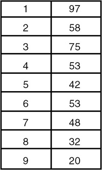
Figure 18.5: A heap.

A heap is definitely not an ordered list because the first entry in the heap has the largest key, and there is no necessary ordering between the keys in locations k and k+1, if k > 1.

A heap is used in sorting a continuous list of length n in O(n log2(n)) comparisons and movements of entries, even in the worst case. The corresponding sorting method is called heapsort.

 

 

SORTING AND SEARCHING

We encounter several applications that require an ordered list. So it is required to order the elements of a given list either in ascending/increasing order or decending/decreasing order, as per the requirement. This process is called sorting. There are many techniques available for sorting an array-based list. These techniques differ in their time and space complexities. Some of the important sorting techniques are discussed here.

 

 

BUBBLE SORT

Introduction

Bubble sorting is a simple sorting technique in which we arrange the elements of the list by forming pairs of adjacent elements. That means we form the pair of the ith and (i+1)th element. If the order is ascending, we interchange the elements of the pair if the first element of the pair is greater than the second element. That means for every pair (list[i],list[i+1]) for i :=1 to (n−1) if list[i] > list[i+1], we need to interchange list[i] and list[i+1]. Carrying this out once will move the element with the highest value to the last or nth position. Therefore, we repeat this process the next time with the elements from the first to (n−1)th positions. This will bring the highest value from among the remaining (n−1) values to the (n−1)th position. We repeat the process with the remaining (n−2) values and so on. Finally, we arrange the elements in ascending order. This requires to perform (n−1) passes. In the first pass we have (n−1) pairs, in the second pass we have (n−2) pairs, and in the last (or (n−1)th) pass, we have only one pair. Therefore, the number of probes or comparisons that are required to be carried out is

and the order of the algorithm is O(n2).

Program

#include #define MAX 10 void swap(int *x,int *y) { int temp; temp = *x; *x = *y; *y = temp; } void bsort(int list[], int n) { int i,j; for(i=0;i<(n-1);i++) for(j=0;j<(n-(i+1));j++) if(list[j] > list[j+1]) swap(&list[j],&list[j+1]); } void readlist(int list[],int n) { int i; printf("Enter the elements "); for(i=0;i

Example

Input

Enter the number of elements in the list, max = 10

5

Enter the elements

23
5
4
9
1

Output

The list before sorting is:

The elements of the list are:

23 5 4 9 1

The list after sorting is:

The elements of the list are:

1 4 5 9 23

 

 

QUICK SORT

Introduction

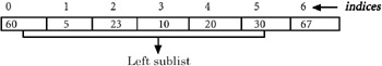
In the quick sort method, an array a[1],…..,a[n] is sorted by selecting some value in the array as a key element. We then swap the first element of the list with the key element so that the key will be in the first position. We then determine the key's proper place in the list. The proper place for the key is one in which all elements to the left of the key are smaller than the key, and all elements to the right are larger.

To obtain the key's proper position, we traverse the list in both directions using the indices i and j, respectively. We initialize i to that index that is one more than the index of the key element. That is, if the list to be sorted has the indices running from m to n, the key element is at index m, hence we initialize i to (m+1). The index i is incremented until we get an element at the ith position that is greater than the key value. Similarly, we initialize j to n and go on decrementing j until we get an element with a value less than the key's value.

We then check to see whether the values of i and j have crossed each other. If not, we interchange the elements at the key (mth)position with the elements at the jth position. This brings the key element to the jth position, and we find that the elements to its left are less than it, and the elements to its right are greater than it. Therefore we can split the list into two sublists. The first sublist is composed of elements from the mth position to the (j–1)th position, and the second sublist consists of elements from the (j+1)th position to the nth position. We then repeat the same procedure on each of the sublists separately.

Choice of the key

We can choose any entry in the list as the key. The choice of the first entry is often a poor choice for the key, since if the list has already been sorted, there will be no element less than the first element selected as the key. So, one of the sublists will be empty. So we choose a key near the center of the list in the hope that our choice will partition the list in such a manner that about half of the elements will end up on one side of the key, and half will end up on the other.

Therefore the function getkeyposition is

int getkeyposition(int i,j)
{
 return(( i+j )/ 2);
}

The choice of the key near the center is also arbitrary, so it is not necessary to always divide the list exactly in half. It may also happen that one sublist is much larger than the other. So some other method of selecting a key should be used. A good way to choose a key is to use a random number generator to choose the position of the next key in each activation of quick sort. Therefore, the function getkeyposition is:

int getkeyposition(int i,j)
{
 return(random number in the range of i to j);
}

Program

#include #define MAX 10 void swap(int *x,int *y) { int temp; temp = *x; *x = *y; *y = temp; } int getkeyposition(int i,int j ) { return((i+j) /2); } void qsort(int list[],int m,int n) { int key,i,j,k; if( m < n) { k = getkeyposition(m,n); swap(&list[m],&list[k]); key = list[m]; i = m+1; j = n; while(i <= j) { while((i <= n) && (list[i] <= key)) i++; while((j >= m) && (list[j] > key)) j-; if( i < j) swap(&list[i],&list[j]); } swap(&list[m],&list[j]); qsort(list[],m,j-l); qsort(list[],j+1,n); } } void readlist(int list[],int n) { int i; printf("Enter the elements "); for(i=0;i

Example

Input

Enter the number of elements in the list, max = 10

10

Enter the elements

7
99
23
11
65
43
23
21
21
77

Output

The list before sorting is:

The elements of the list are:

7 99 23 11 65 43 23 21 21 77

The list after sorting is:

The elements of the list are:

7 11 21 21 23 23 43 65 77 99

Explanation

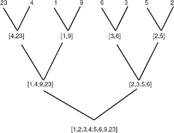
Consider the following list:

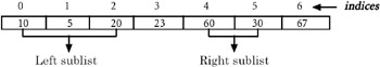
1. When qsort is activated the first time, key = 67, i =1, and j =6. i is incremented until it becomes 7, because there is no element greater than the key. j is not decremented, because at position 6, the value that we have is less than the key. Since i > j, we interchange the key element (the element at position 0) with the element at position 6, and call qsort recursively, with the left sublist made of elements from positions 0 to 5, and the right sublist empty as shown here:

   

2. When qsort is activated the second time on the left sublist as shown, key = 23, i =1, and j =5. i is incremented until it reaches 2. Because the element at position 2 is greater than the key, j is decremented to 4 because the value at position 4 is less than the key. Since i < j, the elements at positions 2 and 4 are swapped. i is then incremeneted to 4 and j is decremented to 3. Since i > j, we interchange the key element (the element at position 0), with the element at position 3, and call qsort recursively with the left sublist made of elements from position 0 to 2, and the right sublist made of elements from position 4 to 5, as shown here:

   

3. By continuing in this fashion, we eventually get the list sorted.
4. The average case-time complexity of the quick sort algorithm can be determined as follows:

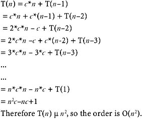
   We assume that every time this is done, the list gets split into two approximately equal-sized sublists. If the size of a given list is n, it gets split into two sublists of size approximately n/2. Each of these sublists gets further split into two sublists of size n/4, and this is continued until the size equals 1. When the quick sort works with a list of size n, it places the key element (which takes the first element of the list under consideration) in its proper position in the list. This requires no more than n iterations. After placing the key element in its proper position in the list of size n, quick sort activates itself twice to work with the left and right sublists, each assumed to be of size n/2. Therefore T(n) is the time required to sort a list of size n. Since the time required to sort the list of size n is equal to the sum of the time required to place the key element in its proper position in the list of size n, and the time required to sort the left and right sublists, each assumed to be of size n/2. T(n) turns out to be:

   ∴ T(n) = c*n + 2*T(n/2)

   where c is a constant and T(n/2) is the time required to sort the list of size n/2.

5. Similarly, the time required to sort a list of size n/2 is equal to the sum of the time required to place the key element in its proper position in the list of size n/2 and the time required to sort the left and right sublists each assumed to be of size n/4. T(n/2) turns out to be:

   T(n/2) = c*n/2 + 2*T(n/4)

   where T(n/4) is the time required to sort the list of size n/4.

   • ∴ T(n/4) = c*n/4 + 2*T(n/8), and so on. We eventually we get T(1) = 1.
   • ∴ T(n) = c*n + 2(c*n(n/2) + 2T(n/4))
   • ∴ T(n) = c*n + c*n + 4T(n/4)) = 2*c*n + 4T(n/4) = 2*c*n + 4(c*(n/4) + 2T(n/8))
   • ∴ T(n) = 2*c*n + c*n + 8T(n/8) = 3*c*n + 8T(n/8)
   • ∴ T(n) = (log n)*c*n + n T(n/n)= (log n)*c*n + n T(1) = n + n*(log n) *c
   • ∴ T(n) μ n log(n)
6. Therefore, we conclude that the average complexity of the quick sort algorithm is O(nlog n). But the worst-case time complexity is of the O(n2). The reason for this is, in the worst case, one of the two sublists will always be empty and the other will be of size (n−1), where n is the size of the original list. Therefore, in the worst case, T(n) turns out to be

   

7. Space complexity: The average-case space complexity is log2n, because the space complexity depends on the maximum number of activations that can exist. We find that if we assume that every time the list gets split into approximately two equal-sized lists, the maximum number of activations that will exist simultaneously will be log2n.

   In the worst case, there exist n activations, because the depth of the recursion is n. So the worst-case space complexity is O(n).

 

 

MERGE SORT

Introduction

This is another sorting technique having the same average-case and worst-case time complexities, but requiring an additional list of size n.

The technique that we use is the merging of the two sorted lists of size m and n to form a single sorted list of size (m + n). Given a list of size n to be sorted, instead of viewing it to be one single list of size n, we start by viewing it to be n lists each of size 1, and merge the first list with the second list to form a single sorted list of size 2.

Similarly, we merge the third and the fourth lists to form a second single sorted list of size 2, and so on. This completes one pass. We then consider the first sorted list of size 2 and the second sorted list of size 2, and merge them to form a single sorted list of size 4.

Similarly, we merge the third and the fourth sorted lists, each of size 2, to form the second single sorted list of size 4, and so on. This completes the second pass.

In the third pass, we merge these adjacent sorted lists, each of size 4, to form sorted lists of size 8. We continue this process until we finally obtain a single sorted list of size n as shown next.

To carry out this task, we require a function to merge the two sorted lists of size m and n to form a single sorted list of size (m + n). We also require a function to carry out one pass of the list to merge the adjacent sorted lists of the specified size. This is because we have to carry out repeated passes of the given list.

In the first pass, we merge the adjacent lists of size 1. In the second pass, we merge the adjacent lists of size 2, and so on. Therefore, we will call this function by varying the size of the lists to be merged.

Program

#include #define MAX 10 void merge(int list[],int list1[],int k,int m,int n) { int i,j; i=k; j = m+1; while( i <= m && j <= n) { if(list[i] <= list[j]) { list1[k] = list[i]; i++; k++; } else { list1[k] = list[j]; j++; k++; } } while(i <= m) { list1[k] = list[i]; i++; k++; } while (i <= n ) { list1[k] = list[j]; j++; k++; } } void mpass( int list[],int list1[],int l,int n) { int i; i = 0; while( i <= (n-2*l+1)) { merge(list,list1,i,(i+l-1),(i+2*l-1)); i = i + 2*l; } if((i+l-1) < n) merge(list,list1,i,(i+l-1),n); else while (i <= n ) { list1[i] = list[i]; i++; } } void msort(int list[], int n ) { int l; int list1[MAX]; l =1; while (l <= n ) { mpass(list,list1,l,n); l = l*2; mpass(list1,list,l,n); l = l*2; } } void readlist(int list[],int n) { int i; printf("Enter the elements "); for(i=0;i

Example

Input

Enter the number of elements in the list, max = 10

10

Enter the elements

11
2
45
67
33
22
11
0
34
23

Output

The list before sorting has the following elements:

11 2 45 67 33 22 11 0 34 23

The list after sorting has the following elements:

0 2 11 11 22 23 33 34 45 67

Explanation

1. The merging of two sublists, the first running from the index 0 to m, and the second running from the index (m + 1) to (n − 1) requires no more than (n−l + 1) iterations.
2. So if l =1, then no more than n iterations are required, where n is the size of the list to be sorted.
3. Therefore, if n is the size of the list to be sorted, every pass that a merge routine performs requires a time proportional to O(n), since the number of passes required to be performed is log2n.
4. The time complexity of the algorithm is O(n log2(n)), for both average-case and worst-case. The merge sort requires an additional list of size n.

 

 

HEAPSORT

Introduction

Heapsort is a sorting technique that sorts a contiguous list of length n with O(n log2 (n)) comparisons and movement of entries, even in the worst case. Hence it achieves the worst-case bounds better than those of quick sort, and for the contiguous list, it is better than merge sort, since it needs only a small and constant amount of space apart from the list being sorted.

Heapsort proceeds in two phases. First, all the entries in the list are arranged to satisfy the heap property, and then the top of the heap is removed and another entry is promoted to take its place repeatedly. Therefore, we need a function that builds an initial heap to arrange all the entries in the list to satisfy the heap property. The function that builds an initial heap uses a function that adjusts the ith entry in the list, whose entries at 2i and 2i + 1 positions already satisfy the heap property in such a manner that the entry at the ith position in the list will also satisfy the heap property.

Program

#include #define MAX 10 void swap(int *x,int *y) { int temp; temp = *x; *x = *y; *y = temp; } void adjust( int list[],int i, int n) { int j,k,flag; k = list[i]; flag = 1; j = 2 * i; while(j <= n && flag) { if(j < n && list[j] < list[j+1]) j++; if( k >= list[j]) flag =0; else { list[j/2] = list[j]; j = j *2; } } list [j/2] = k; } void build_initial_heap( int list[], int n) { int i; for(i=(n/2);i>=0;i-) adjust(list,i,n-1); } void heapsort(int list[],int n) { int i; build_initial_heap(list,n); for(i=(n-2); i>=0;i-) { swap(&list[0],&list[i+1]); adjust(list,0,i); } } void readlist(int list[],int n) { int i; printf("Enter the elements "); for(i=0;i

Example

Input

Enter the number of elements in the list, max = 10

10

Enter the elements

56
1
34
42
90
66
87
12
21
11

Output

The list before sorting is:

The elements of the list are:

56 1 34 42 90 66 87 12 21 11

The list after sorting is:

The elements of the list are:

1 11 12 21 34 42 56 66 87 90

Explanation

In each pass of the while loop in the function adjust(x, i, n), the position i is doubled, so the number of passes cannot exceed log( n/i). Therefore, the computation time of adjust is O(log n/i).

The function build_initial_heap calls the adjust procedure n/2 for values ranging from n1/2 to 0. Hence the total number of iterations will be:

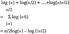
This turns out to be some constant time n. So the computation time of build_initial_heap is O(n). The heapsort function calls the adjust (x,1, i) (n−1) times. So the total number of iterations made in the heapsort will be

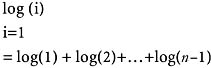
which turns out to be approximately n log(n). So the computing time of heapsort is O(n log(n)) + O(n). The only additional space needed by heapsort is the space for one record to carry out the exchange.

 

 

SEARCHING TECHNIQUES LINEAR OR SEQUENTIAL SEARCH

Introduction

There are many applications requiring a search for a particular element. Searching refers to finding out whether a particular element is present in the list. The method that we use for this depends on how the elements of the list are organized. If the list is an unordered list, then we use linear or sequential search, whereas if the list is an ordered list, then we use binary search.

The search proceeds by sequentially comparing the key with elements in the list, and continues until either we find a match or the end of the list is encountered. If we find a match, the search terminates successfully by returning the index of the element in the list which has matched. If the end of the list is encountered without a match, the search terminates unsuccessfully.

Program

#include #define MAX 10 void lsearch(int list[],int n,int element) { int i, flag = 0; for(i=0;i

Example

Input

Enter the number of elements in the list, max = 10

10

Enter the elements

23
1
45
67
90
100
432
15
77
55

Output

The list before sorting is:

The elements of the list are:

23 1 45 67 90 100 432 15 77 55

Enter the element to be searched

100

The element whose value is 100 is present at position 5 in list

Input

Enter the number of elements in the list max = 10

10

Enter the elements

23
1
45
67
90
101
23
56
44
22

Output

The list before sorting is:

The elements of the list are:

23 1 45 67 90 101 23 56 44 22

Enter the element to be searched

100

The element whose value is 100 is not present in the list

Explanation

1. In the best case, the search procedure terminates after one comparison only, whereas in the worst case, it will do n comparisons.
2. On average, it will do approximately n/2 comparisons, since the search time is proportional to the number of comparisons required to be performed.
3. The linear search requires an average time proportional to O(n) to search one element. Therefore to search n elements, it requires a time proportional to O(n2).
4. We conclude that this searching technique is preferable when the value of n is small. The reason for this is the difference between n and n2 is small for smaller values of n.

 

 

BINARY SEARCH

Introduction

The prerequisite for using binary search is that the list must be a sorted one. We compare the element to be searched with the element placed approximately in the middle of the list.

If a match is found, the search terminates successfully. Otherwise, we continue the search for the key in a similar manner either in the upper half or the lower half. If the elements of the list are arranged in ascending order, and the key is less than the element in the middle of the list, the search is continued in the lower half. If the elements of the list are arranged in descending order, and the key is greater than the element in the middle of the list, the search is continued in the upper half of the list. The procedure for the binary search is given in the following program.

Program

#include #define MAX 10 void bsearch(int list[],int n,int element) { int l,u,m, flag = 0; l = 0; u = n-1; while(l <= u) { m = (l+u)/2; if( list[m] == element) { printf(" The element whose value is %d is present at position %d in list ", element,m); flag =1; break; } else if(list[m] < element) l = m+1; else u = m-1; } if( flag == 0) printf("The element whose value is %d is not present in the list ", element); } void readlist(int list[],int n) { int i; printf("Enter the elements "); for(i=0;i

Example

Input

Enter the number of elements in the list, max = 10

10

Enter the elements

34
2
1
789
99
45
66
33
22
11

Output

The elements of the list before sorting are:

34 2 1 789 99 45 66 33 22 11
1 2 3 4 5 6 7 8 9 10

Enter the element to be searched

99

The element whose value is 99 is present at position 5 in the list

Input

Enter the number of elements in the list max = 10

10

Enter the elements

54
89
09
43
66
88
77
11
22
33

Output

The elements of the list before sorting are:

54 89 9 43 66 88 77 11 22 33

Enter the element to be searched

100

The element whose value is 100 is not present in the list.

In the binary search, the number of comparisons required to search one element in the list is no more than log2n, where n is the size of the list. Therefore, the binary search algorithm has a time complexity of O(n *( log2n.).)

 

 

HASHING

Introduction

A data object called a symbol table is required to be defined and implemented in many applications, such as compiler/assembler writing. A symbol table is nothing but a set of pairs (name, value), where value represents a collection of attributes associated with the name, and the collection of attributes depends on the program element identified by the name.

For example, if a name x is used to identify an array in a program, then the attributes associated with x are the number of dimensions, lower bound and upper bound of each dimension, and element type. Therefore, a symbol table can be thought of as a linear list of pairs (name, value), and we can use a list data object for realizing a symbol table.

A symbol table is referred to or accessed frequently for adding a name, or for storing or retrieving the attributes of a name.

Therefore, accessing efficiency is a prime concern when designing a symbol table. The most common method of implementing a symbol table is to use a hash table.

Hashing is a method of directly computing the index of the table by using a suitable mathematical function called a hash function.

Note 

The hash function operates on the name to be stored in the symbol table, or whose attributes are to be retrieved from the symbol table.

If h is a hash function and x is a name, then h(x) gives the index of the table where x, along with its attributes, can be stored. If x is already stored in the table, then h(x) gives the index of the table where it is stored, in order to retrieve the attributes of x from the table.

There are various methods of defining a hash function. One is the division method. In this method, we take the sum of the values of the characters, divide it by the size of the table, and take the remainder. This gives us an integer value lying in the range of 0 to (n−1), if the size of the table is n.

Another method is the mid-square method. In this method, the identifier is first squared and then the appropriate number of bits from the middle of the square is used as the hash value. Since the middle bits of the square usually depend on all the characters in the identifier, it is expected that different identifiers will result in different values. The number of middle bits that we select depends on the table size. Therefore, if r is the number of middle bits that we are using to form the hash value, then the table size will be 2r. So when we use this method, the table size is required to be a power of 2.

A third method is folding, in which the identifier is partitioned into several parts, all but the last part being of the same length. These parts are then added together to obtain the hash value.

To store the name or to add attributes of the name, we compute the hash value of the name, and place the name or attributes, as the case may be, at that place in the table whose index is the hash value of the name.

To retrieve the attribute values of the name kept in the symbol table, we apply the hash function of the name to that index of the table where we get the attributes of the name. So we find that no comparisons are required to be done; the time required for the retrieval is independent of the table size. The retrieval is possible in a constant amount of time, which will be the time taken for computing the hash function.

Therefore a hash table seems to be the best for realization of the symbol table, but there is one problem associated with the hashing, and that is collision.

Hash collision occurs when the two identifiers are mapped into the same hash value. This happens because a hash function defines a mapping from a set of valid identifiers to the set of those integers that are used as indices of the table.

Therefore we see that the domain of the mapping defined by the hash function is much larger than the range of the mapping, and hence the mapping is of a many-to-one nature. Therefore, when we implement a hash table, a suitable collision-handling mechanism is to be provided, which will be activated when there is a collision.

Collision handling involves finding an alternative location for one of the two colliding symbols. For example, if x and y are the different identifiers and h(x = h(y), x and y are the colliding symbols. If x is encountered before y, then the ith entry of the table will be used for accommodating the symbol x, but later on when y comes, there is a hash collision. Therefore we have to find a suitable alternative location either for x or y. This means we can either accommodate y in that location, or we can move x to that location and place y in the ith location of the table.

Various methods are available to obtain an alternative location to handle the collision. They differ from each other in the way in which a search is made for an alternative location. The following are commonly used collision-handling techniques:

Linear Probing or Linear Open Addressing

In this method, if for an identifier x, h(x) = i, and if the ith location is already occupied, we search for a location close to the ith location by doing a linear search, starting from the (i+1)th location to accommodate x. This means we start from the (i+1)th location and do the linear search until we get an empty location; once we get an empty location we accommodate x there.

Rehashing

In rehashing we find an alternative empty location by modifying the hash function and applying the modified hash function to the colliding symbol. For example, if x is the symbol and h(x) = i, and if the ith location is already occupied, then we modify the hash function h to h1, and find out h1(x), if h1(x) = j. If the jth location is empty, then we accommodate x in the jth location. Otherwise, we once again modify h1 to some h2 and repeat the process until the collision is handled. Once the collision is handled, we revert to the original hash function before considering the next symbol.

Overflow chaining

Overflow chaining is a method of implementing a hash table in which the collisions are handled automatically. In this method, we use two tables: a symbol table to accommodate identifiers and their attributes, and a hash table, which is an array of pointers pointing to symbol table entries. Each symbol table entry is made of three fields: the first for holding the identifier, the second for holding the attributes, and the third for holding the link or pointer that can be made to point to any symbol table entry. The insertions into the symbol table are done as follows:

If x is the symbol to be inserted, it will be added to the next available entry of the symbol table. The hash value of x is then computed. If h(x) = i, then the ith hash table pointer is made to point to the symbol table entry in which x is stored, if the ith hash table pointer does not point to any symbol table entry. If the ith hash table pointer is already pointing to some symbol table entry, then the link field of the symbol table entry containing x is made to point to that symbol table entry to which the ith hash table pointer is pointing to, and the ith hash table pointer is made to point to the symbol entry containing x. This is equivalent to building a linked list on the ith index of the hash table. The retrieval of attributes is done as follows:

If x is a symbol, then we obtain h(x), use this value as the index of the hash table, and traverse the list built on this index to get that entry which contains x. A typical hash table implemented using this technique is shown here.

The symbols to b stored are x1,y1,z1,x2,y2,z2. The hash function that we use is h(symbol) = (value of first letter of the symbol) mod n, where n is the size of table.

if h(x1) = i

h(y1) = j
h(z1) = k

then

h(x2) = i
h(y2) = j
h(z2) = k

Therefore, the contents of the symbol table will be the one shown in Figure 18.6.

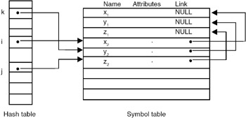
Figure 18.6: Hash table implementation using overflow chaining for collision handling.

 

 

HASHING FUNCTIONS

Some of the methods of defining a hash function are discussed in the following paragraphs.

Modular Arithmetic

In modular arithmetic, first the key is converted to an integer, then it is divided by the size of the index range, and the remainder is taken to be the hash value. The spread achieved depends very much on the modulus. If the modulus is the power of small integers such as 2 or 10, then many keys tend to map into the same index, while other indices remain unused. The best choice for the modulus is often, but not always, a prime number, which usually has the effect of spreading the keys quite uniformly.

Truncation

Truncation ignores part of the key, and uses the remainder directly as the hash value (using numeric code to represent non-numeric field data). If the keys, for example, are eight-digit numbers and the hash table has 1000 entries, then the first, second, and fifth digits from the right side might make the hash value. So, 62538194 maps to 394. It is a fast method, but it often fails to distribute keys evenly.

Folding

In folding, the identifier is partitioned into several parts, all but the last part being of the same length. These parts are then added together to obtain the hash value. For example, an eight-digit integer can be divided into groups of three, three, and two digits. The groups are then added together, and truncated, if necessary, to be in the proper range of indices. So 62538149 maps to 625 + 381 + 94 = 1100, truncated to 100. Since all information in the key can affect the value of the function, folding often achieves a better spread of indices than truncation.

Mid-square method

In this method, the identifier is squared (using numeric code to represent non- numeric field data), and then the appropriate number of bits from the middle of the square are used to get the hash value. Since the middle bits of the square usually depend on all the characters in the identifier, it is expected that different identifiers will result in different values. The number of middle bits that we select depends on table size. Therefore, if r is the number of middle bits used to form the hash value, then the table size will be 2r. So when we use the mid- square method, the table size should be a power of 2.

Program

A complete C program for implementation of a hash table is given here:

#include 
#include 
#include 
#define SIZE 50
#define MAX 10
 typedef struct node
 {
 char symbol[MAX];
 int value;
 struct node *next;
 } entry;
 typedef entry *entry_ptr;

 int hash_value(char * name)
 {
 int sum=0;
 while( *name != '')
 {
 sum += *name;
 name++;
 }
 return(sum % SIZE);
 }
 void initialize( entry_ptr table[])
 {
 int i=0;
 for(i=0; isymbol,name) == 0)
 {
 printf("The symbol %s is already present in the
table
",name);
 flag =0;;
 }
 temp=temp->next;
 }
 if(flag)
 {
 temp = (entry_ptr) malloc(sizeof( entry));
 if(temp == NULL)
 {
 printf("ERRRR .......
");
 exit(0);
 }
 strcpy(temp->symbol,name);
 temp->value = val;
 temp->next = table[h];
 table[h]=temp;
 }
 }
 void retrieve( entry_ptr table[],char *name)
{
 int h,flag =1;
 entry_ptr temp;
 h = hash_value(name);
 temp = table[h];
 while( temp != NULL && flag)
{
 if( strcmp(temp->symbol,name) == 0)
 {
printf("The symbol %s is present in the table and having value =
%d
",
 name,temp->value);
 flag =0;
 }
 temp=temp->next;
 }
 if(flag == 1)
 printf("The symbol %s is not present in the table

",name);
 }
 void main()
 {
 entry_ptr table[SIZE];
 char name[MAX];
 int value,n;
 initialize(table);
 do
 {
 do
{
 printf("Enter the symbol and value pair to be inserted
");
 scanf("%s %d",name,&value);
 insert(table,name,value);
 printf("Enter 1 to continue
");
 scanf("%d",&n);
}
while(n == 1);
do
{
 printf("Enter the symbol whose value is to be retrieved
");
 scanf("%s",name);
 retrieve(table,name);
 printf("Enter 1 to continue
");
 scanf("%d",&n);
}while( n == 1);
 printf("Eneter 1 to continue
");
 scanf("%d",&n);
 }while(n == 1);
}

Example

Input and Output

Enter the symbol and value pair to be inserted

ogk10

Enter 1 to continue

1

Enter the symbol and value pair to be inserted

psd20

Enter 1 to continue

0

Enter the symbol whose value is to be retrieved

ogk

The symbol ogk is present in the table with the value = 10

Enter 1 to continue

1

Enter the symbol whose value is to be retrieved

psd

The symbol psd is present in the table with the value = 20

Enter 1 to continue

1

Enter the symbol whose value is to be retrieved

asg

The symbol asg is not present in the table

Enter 1 to continue

0

Eneter 1 to continue

1

Enter the symbol and value pair to be inserted

asg30

Enter 1 to continue

0

Enter the symbol whose value is to be retrieved

asg

The symbol asg is present in the table with the value = 30

Enter 1 to continue

0

Eneter 1 to continue

0

Exercises

1. Consider an unsorted array A[n] of integer elements that may have many elements present more than once. It is required to store only the distinct elements of the array A in a separate array B. The information about the number of times each element is replicated is maintained in a third array C. For example, C[0] would indicate the number of times the element B[0] occurs in array A. Write a C program to generate the arrays B and C, given an array A.
2. Write a C program that finds the largest and the second largest elements in an unsorted array A. The program should make just a single scan of the array.
3. Sort the following list by applying the bubble sort method.

   10
   01
   11
   100
   23
   21
   11
   99
   78
   

4. Sort the following list by applying the heapsort method.

   44
   23
   67
   88
   22
   43
   90
   04
   

5. Consider the following list whose elements are arranged in ascending order. Assume that a binary search technique is used. Determine the number of probes required to find each entry in the list.

   11
   22
   43
   56
   67
   71
   89