Writing Advanced Queries and Subqueries

Understanding the Restrictions on Subqueries Used as Predicates for a Comparison Operator

Many queries use a comparison operator within the WHERE clause to select rows in which one or more columns have a particular value or range of values. For example, to display a list of employees hired after 2/1/2002 you might use the query:

 SELECT first_name, last_name
 FROM employees
 WHERE hire_date > '2/1/2002'

Similarly, to list the chemistry grades for all students from California you might use a query such as:

 SELECT first_name, last_name, grade
 FROM students AS s, grades AS g
 WHERE s.home_state = 'CA'
 AND s.student_ID = g.student_ID
 AND g.class = 'chemistry'

While the substance of the two queries differs, the WHERE clauses are similar in that they both have comparison operators nestled between a pair of scalar values. In fact, a comparison operator (=, <>, >, <, >=, or <=) can only be used to compare two scalar values—a scalar value to the left of the operator with the value to the right of the operator. However, unlike the comparisons made in the two preceding examples, you don't always know the scalar values you want to use within the comparison when you write a query. Fortunately, you can use a subquery (either correlated or uncorrelated) in place of the scalar value on either or both sides of a comparison operator.

The restriction on using a subquery in place of a scalar value is that the subquery must return one value at most. That is, the SELECT statement in the subquery must return a results set that consists of either zero or one row with only one column. SQL programmers often refer to subqueries that return a scalar value as scalar subqueries.

To make a list of students with GPAs 25 percent greater than the average GPA, you might write the following query:

 SELECT first_name, last_name, gpa
 FROM students
 WHERE gpa > ((SELECT AVG(gpa) FROM students) * 1.25)

Without knowing the average GPA, you can still write the query that selects rows based on its value by using an uncorrelated, scalar subquery (which follows the greater than [>] comparison operator) to compute it when the DBMS executes the query. Because the subquery in this example is uncorrelated, the DBMS need only execute it once. An uncorrelated subquery would return the same results set no matter how many times it is called during the query. In this example, the optimizer reduces it to a constant value before scanning the tables listed in the FROM clause within the query—STUDENTS.

You are not limited to using only uncorrelated subqueries with comparison operators. Although the processing is a bit more complex (for the DMBS), you can use correlated subqueries as well. Suppose, for example, that you want a list of realtors that have sold homes with an average sale price of $500,000 or more. You might write the query as:

 SELECT first_name, last_name
 FROM realtors AS r
 WHERE 500000.00 <= (SELECT AVG(sales_price)
 FROM sales AS s
 WHERE s.realtor_ID = r.realtor_ID)

In this example, the DBMS must execute the correlated subquery repeatedly—once for each realtor as the DBMS scans the REALTORS table. Each time the DBMS executes it, the correlated subquery returns a single (albeit, different), value. (To be a legal predicate for an unmodified comparison operator, a subquery must return a scalar value.)

Using a VIEW to Allow a Self Join on the Working Table in a Subquery

Typically, multi-table queries involve a relationship between two or more tables. Suppose, for example, that you want to list all customers that purchased a red Corvette. You might write the following query that relates personal information within the CUSTOMERS table with purchase data within the SALES table:

 SELECT first_name, last_name, date_sold, price
 FROM customers AS c, sales AS s
 WHERE c.cust_ID = s.sold_to
 AND make='Corvette'
 AND color='red'

Sometimes, however, you want to write a mutli-table query that involves a relationship with itself. Suppose, for example, that you want to list all employees that have been with the company longer than their managers. When executing the query, the DBMS must compare column values from one row within a table to column values within another row of the same table. In Tip 313, "Using a Table Alias to do a Single-Table JOIN (i.e. Self-JOIN)," you learned how to write multi-table queries that involve relationships within a single table. To write the query in this example, you might use the following SELECT statement:

 SELECT e.emp_ID, e.first_name, e.last_name,
 e.date_hired AS 'Employee Hired',
 m.emp_ID AS 'Manager ID', m.date_hired AS 'Manager Hired'
 FROM employees AS e, employees AS m
 WHERE e.manager_ID = m.emp_ID
 AND e.date_hired < m.date_hired

By assigning correlation names ("e" and "m") to the EMPLOYEES table, you make it possible for the DBMS to perform a self-join. In a self-join, the DBMS works with the rows within a table as if it were working with rows from two separate tables—table "e" and table "m," in this example. The DBMS joins rows from the EMPLOYEES table "e" with rows from the EMPLOYEES table "m" and returns column values from those (virtual) joined rows in which the column values satisfy the search criteria in the query's WHERE clause.

Unfortunately, not all SQL statements let you use a correlation name for the target table. Suppose, for example, that you want to reduce the salary of any employee by 25 percent. The employee was hired prior to his or her manager. Although it seems to express (in SQL terms) the update you want to perform, the following UPDATE statement is syntactically incorrect—an UPDATE statement does not let you specify a correlation name in its UPDATE clause as shown here:

 UPDATE employees AS m SET salary = salary * 0.75
 WHERE employees.manager_ID = m.emp_ID
 AND e.date_hired < m.date_hired

To eliminate the invalid correlation name "m" in this UPDATE statement, you can create on the EMPLOYEES table a VIEW that lists all managers. Then, you can use the VIEW as a second table for the subquery within the UPDATE statement's WHERE clause.

Suppose, for example, that all non-management employees have a non-null value in the MANAGER_ID column whereas managers do not. The following VIEW will then return a list of all managers:

 CREATE vw_managers
 AS SELECT * FROM employees WHERE manager_ID IS NULL

Given the VW_MANAGERS VIEW, which returns the DATE_HIRED and EMP_ID for the management employees, you could write the preceding UPDATE statement as:

UPDATE employees SET salary = salary * 0.75
WHERE EXISTS (SELECT *
 FROM vw_managers AS m
 WHERE employees.manager_ID = m.emp_ID
 AND employees.date_hired < m.date_hired)

Note 

Some DBMS products (such as MS-SQL Server, for example) let you reference the UPDATE (or DELETE) statement's target table within a subquery without listing the table within the subquery's FROM clause. As such, you need not create a VIEW to make an outer reference to the target table within the subquery on these DBMS platforms. On MS-SQL Server for example, you can write the UPDATE statement in the preceding example without using a VIEW as:

UPDATE employees SET salary = salary * 0.75
WHERE EXISTS (SELECT *
 FROM employees AS m
 WHERE employees.manager_ID = m.manager_ID
 AND employees.date_hired < m.date_hired)

MS-SQL Server will correctly use values from the outer reference to columns within the EMPLOYEES table in the statement's UPDATE clause when making comparisons with column values (from the same table) within the subquery's WHERE clause.

Using a Temporary Table to Remove Duplicate Data

If you create a table without a PRIMARY KEY or at least one column constrained as both UNIQUE and NOT NULL, users can (and according to Murphy's law, probably will) insert duplicate rows of data. Duplicate relations (that is, duplicate rows) within a table are seldom, if ever, desirable. Duplicate data not only takes up extra space and increases retrieval time and memory usage, but also prevents you from normalizing the database. To prevent database corruption due to DELETE, INSERT, and UPDATE anomalies, you must normalize the database, which, you learned to do in Tips 200–203.

The first step in the normalization process is to put all database tables into first normal form (1NF). (You learned about 1NF in Tip 201 "Understanding First Normal Form [1NF].") Because one of the requirements of 1NF is that a table has no duplicate rows, eliminating duplicate data will be one or your first tasks on the road to the desired, anomaly-free third normal form (3NF).

Unfortunately, deleting duplicate data is not as simple as executing a DELETE statement with the appropriate WHERE clause. Remember, when executed, a DELETE statement will remove all rows that satisfy the search conditions within its WHERE clause. Thus, the DELETE statement that eliminates one row of duplicate data will remove all duplicate rows—without leaving the desired one (now non-duplicated) row in the table.

One way to delete all but one row from each set of duplicate rows is to perform the following steps:

1. Create a temporary table with the same structure as the table that contains the duplicate data.
2. Use an INSERT statement that has a SELECT statement with a DISTINCT clause to move rows from the table with duplicate data into a new, temporary table.
3. Truncate (that is, drop all rows within) the original table.
4. Use the ALTER TABLE statement to add a UNIQUE constraint, which will prevent the insertion of duplicate rows in the future.
5. Use an INSERT statement that has a SELECT statement to copy all rows from the temporary table back into the (now) empty, original table.
6. Drop the temporary table.

Suppose, for example, that you had a table name ITEMS with the following structure:

 ITEM_NUMBER INTEGER
 DESCRIPTION VARCHAR(45)
 COST MONEY

To remove duplicates from the ITEMS table, you might execute the following statement batch:

 /* Create a temporary table */
 CREATE TABLE #temp_items
 (item_number INTEGER,
 description VARCHAR(45),
 cost MONEY)

 /* Use the DISTINCT clause to prevent the INSERT statement
 from putting duplicate data into the temporary table */

 INSERT INTO #temp_items
 SELECT DISTINCT * FROM items

 /* Delete all rows from the ITEMS table */

 TRUNCATE TABLE items

 /* (Optional) - Apply a uniqueness constraint to the
 original table to prevent future duplicates /

 ALTER TABLE items ADD UNIQUE (item_number)

 /* Return data from the temporary data */

 INSERT INTO items
 SELECT * FROM #temp_items

 /* Drop the temporary table */

 DROP #temp_items

Note 

If the table with the duplicate data has any FOREIGN KEY constraints with an ON DELETE CASCADE rule or if the table has a DELETE or INSERT trigger, make sure you turn them all off before you start the duplicate row removal procedure. After moving the data from the temporary table back into the original table, turn the constraints and triggers back on.

Using a Temporary Table to Delete Rows from Multiple Tables

All commercially available DMBS products support referential integrity constraints that let the user setup parent/child relationships between pairs of tables. A referential integrity constraint requires that a FOREIGN KEY value in a child table must have a matching PRIMARY KEY value within the parent table. However, some DBMS products do not yet support DELETE triggers or the ON DELETE CASCADE referential integrity rule. Without these features, it can be difficult to delete rows from the parent table when some or all the parent table's rows are referenced by FOREIGN KEY values within rows of one or more child tables. To maintain referential integrity, you must first delete the child rows before you delete a child row's parent row.

A DELETE trigger is nothing more than a stored procedure the DBMS executes when you attempt to delete a row from the table to which you attached the trigger. What makes a trigger more handy than a stored procedure in this instance is that the DBMS executes the trigger's statements before deleting the row from the table to which the trigger is attached (as you learned in Tip 451 "Understanding DELETE Triggers"). Thus, by using a DELETE trigger you can have the DBMS delete child rows (in one or more tables) before deleting the parent row—even though you submit to the DBMS only the DELETE statement that removes one or more rows from the parent table.

Similarly, if your DMBS supports it, you can apply the ON DELETE CASCADE rule to FOREIGN KEY constraints and have the DBMS delete any child rows whenever you delete a parent row from the table with the PRIMARY KEY referenced by the child's FOREIGN KEY. (You learned how the ON DELETE CASCADE rule works in Tip 183 "Understanding How Applying the CASCADE Rule to Updates and Deletes Helps Maintain Referential Integrity.")

If your DBMS supports neither DELETE triggers nor the ON DELETE CASCADE rule for FOREIGN KEY constraints, you can still delete rows from multiple tables. Simply build a temporary table with the list of rows you want to delete before executing the necessary DELETE statements to remove corresponding rows from child tables and then from the parent table. You might also use the following method to DELETE "child" rows from tables in which you have not used FOREIGN KEY references to setup explicit parent/child relationships.

To delete rows from multiple tables without referential integrity (or DELETE triggers), perform the following steps:

1. Create a temporary table in which to hold the key (usually PRIMARY KEY) values you can use to identify "child" rows you want to delete in other tables.
2. Use a SELECT statement to insert the key values into the temporary table.
3. Use a DELETE statement with a subquery in its WHERE clause to delete the child rows from each of the related tables.
4. Use a DELETE statement with a subquery in its WHERE clause to delete from the parent table the rows identified by the key values within the temporary table.
5. DROP the temporary table.

Suppose, for example, that your company sends a free gift to customers along with the products they ordered. If the company later decides to discontinue the free gift products, you must remove them from the ITEM_MASTER, INVENTORY, and ORDERS tables. To do so, you might execute the following statement batch to delete rows from all three tables as a single transaction:

 /* Create a temporary table */
 CREATE TABLE #temp_discontinued
 (item_number INTEGER)

 /* Use the DISTINCT clause to prevent the INSERT statement
 from putting duplicate data into the temporary table */
 INSERT INTO #temp_discontinued
 SELECT DISTINCT item_number
 FROM item_master WHERE type = 'gift'

 /* Delete child rows from related tables */

 DELETE FROM inventory
 WHERE item_no IN (SELECT item_number
 FROM #temp_discontinued)
 DELETE FROM orders
 WHERE item_no IN (SELECT item_number
 FROM #temp_discontinued)

 /* Delete the "parent" row from the parent table */

 DELETE FROM item_master
 WHERE item_number IN (SELECT item_number
 FROM #temp_discontinued)

 /* Drop the temporary table */

 DROP #temp_discontinued

Although executing the same subquery multiple times may appear inefficient, bear in mind that the DBMS optimizer reviews all the statements in a statement batch and creates an execution plan prior to executing them. When the optimizer sees the same subquery used repeatedly, the optimizer executes the subquery only once and then uses subquery's (virtual) results table (without re-executing the subquery) each time the subquery appears within the statement batch.

Note 

Although you could execute the following DELETE statement at the end of the statement batch to remove the gift items from the ITEM_MASTER table, it is better to use the subquery, as shown in the example instead:

DELETE FROM item_master WHERE type = 'gift'

By using the same, static subquery results table for all DELETE statements, you avoid the possibility of removing items from the ITEM_MASTER that you have not removed from its child tables. For example, if a user marks additional items as gift after the DBMS executes INSERT statement within the statement batch to build the #TEMP_DISCONTINUED table, executing the preceding DELETE statement would cause the DBMS to delete items from the ITEM_MASTER that it has not yet deleted from its child tables.

Using the UPDATE Statement to Set the Values in One Table Based on the Values in a Second Table

Unless you are performing maintenance operations or correcting inaccurate data values within a table, you typically use a data-entry program to accept new data or changes to existing data from database users. As a result, most UPDATE statements you write will be simple expressions that set the value of a column to the number or character string the user entered into a data entry field within an application program. If the user entered a number, you might set a column's value based on the results of a mathematical formula involving a column's current value and the number the user entered. As such, most UPDATE statements will be of the form:

 UPDATE 
 SET  = 
 WHERE 

However, you are not limited to this simple form for the UPDATE statement. For example, there is no rule against placing a column name on both sides of the equal sign. While the following UPDATE statement does not actually change the column's value, you can use it to trigger referential integrity actions. This can happen if the column being "updated" is a PRIMARY KEY referenced by a FOREIGN KEY with an ON UPDATE rule. You can also use it to execute a trigger if there is an UPDATE trigger on the column or on the table:

 UPDATE customers SET cust_no = cust_no

In addition, you are not limited to using only a column name, variable, literal, or simple expression on the right of any equal sign (=) within an UPDATE statement's SET clause. You can also set a column to the value returned by a scalar subquery (that is, a subquery that returns a single, scalar value). Moreover, the UPDATE statement's WHERE clause can also contain a subquery, so long as the subquery is part of an expression that returns a TRUE or FALSE result.

For example, you might use a subquery within a SET clause (and within the WHERE clause) to write an UPDATE statement that collects summary data about one table and posts it to rows within another table. Suppose, for example, that you have CUSTOMERS, UNPOSTED_PAYMENTS, and PAYMENT_HISTORY tables. To update each customer's ACCOUNT_BALANCE and AVERAGE_PAYMENT data (within the CUSTOMERS table), you could execute the following statement batch:

 /* Mark the payments to be posted and insert them into the
 payment history table */

 UPDATE unposted_payments SET post = 'Y'
 INSERT INTO payment_history SELECT * FROM unposted_payments
 WHERE post = 'Y'
 /* Execute the UPDATE statement that posts the unposted
 payments marked for posting */

 UPDATE customers
 SET account_balance = account_balance -
 (SELECT SUM(amount_paid)
 FROM unposted_payments AS up
 WHERE customers.cust_ID = up.cust_ID),

 average_payment =
 (SELECT avg(amount_paid)
 FROM payment_history as ph
 WHERE customers.cust_ID = ph.cust_ID)

 WHERE EXISTS (SELECT *
 FROM unposted_payments as up
 WHERE customers.cust_ID = up.cust_ID
 AND up.post = 'Y' )

 /* Remove posted payments from the unposted payments
 table */

 DELETE FROM unposted_payments WHERE post = 'Y'

As mentioned previously within this tip, each SELECT statement used in the UPDATE statement's SET clause must return a single scalar value. This example uses aggregate functions to ensure a scalar result. Although you might be tempted to write the SELECT clause in the first subquery as "SELECT amount_paid," it could be a mistake. If a customer makes more than one payment, "SELECT amount_paid" will return multiple values, and the entire UPDATE process would fail.

Note, too, that the UPDATE statement's WHERE clause uses a subquery to determine if there are any unposted payments from the customer. If not, the DBMS need not compute the average payment, since there can be no change to the average payment already within the AVERAGE_PAYMENT column of the CUSTOMERS table. More importantly, checking for the existence of payments also ensures that the AVG() aggregate will not return a NULL value. AVG() would return a NULL value if there were no payments from a customer and the subquery passed an empty table to the aggregate.

The scalar subqueries in this example are able to select payments from a particular customer, because a table referenced in the UPDATE clause is available for use throughout the remaining clauses within the UPDATE statement. Therefore, column values from the current row within the CUSTOMERS table are available for use throughout all the UPDATE statement's subqueries.

Optimizing the EXISTS Predicate

To check if a column (or literal) value is within a list of values, use an IN predicate. For example, if you want a list of all customers whose salesperson was either Mary, Mark, or Sue, you would use an IN predicate such as that in the following query:

 SELECT * FROM customers
 WHERE salesperson IN ('Mary', 'Mark', 'Sue')

Rather than list values individually, you can use a subquery to build the list of possible values you want to check. For example, to remove the phone numbers of all the current customers from the PROSPECTS list, you might write the following DELETE statement:

 DELETE FROM prospects
 WHERE phone_number IN (SELECT phone_number FROM customers)

When you want to perform an action when there is at least one item within a results set, use the EXISTS predicate. For example, in Tip 550, "Using the UPDATE Statement to Set the Values in One Table Based on the Values in a Second Table," you want the DBMS to update the customer account balance and average payment data if there is at least one payment from the customer within the UNPOSTED_PAYMENTS table. If you had only wanted to execute the UPDATE statement if the customer made a payment of a particular amount, you might have written the UPDATE statement's WHERE clause as:

 WHERE customer.normal_payment IN
 (SELECT amount_paid
 FROM unposted_payments AS up
 WHERE customers.cust_ID = up.cust_ID
 AND up.post = 'Y')

However, since you were not checking for a specific AMOUNT_PAID and wanted the DBMS to execute the UPDATE statement if the UNPOSTED_PAYMENTS table contained a payment in any amount from the customer, you can use the EXISTS predicate in the statement's WHERE clause as:

 WHERE EXISTS (SELECT *
 FROM unposted_payments as up
 WHERE customers.cust_ID = up.cust_ID
 AND up.post = 'Y')

As you will learn from the following discussion, there are three ways you can write an EXISTS predicate, and the one you choose depends on your DBMS platform. To decide which is the optimum EXISTS predicate for your DMBS platform, try executing the same query using each the three forms. Use the one that your DBMS optimizer reports as the "least costly." When you submit a query, the DBMS optimizer generates an execution plan. You learned how to review a statement's execution plan in Tip 524 "Understanding the MS-SQL Server SHOWPLAN_ALL Option for Displaying Statement Execution Plans and Statistics."

In SQL-89, the rule was that the subquery used in an EXISTS predicate had to have a SELECT clause which contained either a single column or an asterisk (*). When you used SELECT *, the DBMS (at least in theory) picked one of the columns from the tables listed in the SELECT statement's FROM clause and used it. (Remember, when you use an EXISTS predicate you are not looking for a specific value of any particular type; you are just checking to see if the subquery returns any value at all.)

SQL-92, which can handle row-valued comparison, no longer restricts you to listing only a single column or asterisk (*) in the EXISTS predicate's subquery. However, as of this writing, most DBMS products still do not support row-valued comparisons. Thus, the three most popular forms for the EXISTS predicate are:

• EXISTS (SELECT * FROM

 WHERE )

• EXISTS (SELECT FROM

 WHERE )

• EXISTS (SELECT FROM

 WHERE )

In general, the first form, SELECT * FROM ... should work better than specifying either a column name or constant value. SELECT * FROM ... lets the optimizer decide which column to use. As such, if there is an INDEX on the column used in the subquery's WHERE clause, the optimizer can use the indexed column and never have to touch the table data at all. In the preceding example, if there is an index on the CUST_ID column of the UNPOSTED_PAYMENTS table, the DBMS need only check the index (on CUST_ID). Indexes are typically smaller than tables and structured for very fast searching. If the DBMS finds the value within the index, the EXISTS predicate is true; if the value is not in the index, the predicate is FALSE. In either case, the DBMS need not retrieve actual values from the UNPOSTED_PAYMENTS table.

Although SELECT * FROM ... should, in theory, be the optimal form of the EXISTS predicate, some DBMS products will actually execute the subquery and build a "virtual" table of query results. In other words, instead of just check for a value within any one of the table's columns, the DBMS builds an in-memory table that contains the values from all columns within rows that satisfy the subquery's search criteria. On such systems, limiting the results table to a single column by using the SELECT form of the EXISTS predicate is better than having the DBMS build a multi-column, multi-row interim table.

Finally, you should use the third form of the EXISTS predicate (SELECT ) on those DBMS products, like Oracle, that must be told they do not have to retrieve the actual column values when building the subquery's virtual table. If you supply a literal (constant) value, the DBMS simply repeats that value for each row that satisfies the subquery's search criteria. Although, the DBMS still has to scan the subquery's base table, it does not have to retrieve the actual data values from table columns into memory.

Using the ALL Predicate to Combine Two Queries into One

In Tip 546 "Understanding the Restrictions on Subqueries Used as Predicates for a Comparison Operator," you learned that you can use a subquery as one of the values in a comparison—as long as the subquery returns a single scalar value. Thus, you can use a scalar subquery (that is, a subquery that returns a scalar value) to execute queries such as the following, which lists the names and total sales for the employees with the highest TOTAL_SALES within the EMPLOYEES table:

 SELECT first_name, last_name, total_sales
 FROM employees
 WHERE total_sales = (SELECT MAX(total_sales)
 FROM employees)

SQL provides three quantifiers (sometimes called qualifiers) that let you use subqueries that return a set of (multiple) values in a comparison. The quantifiers are ALL, SOME, and ANY. A quantifier then, is a logical operator that asserts the quantity of objects for which a statement (in this case a comparison) is TRUE. Thus, you could rewrite the preceding query as:

 SELECT first_name, last_name, total_sales
 FROM employees
 WHERE total_sales >= ALL (SELECT total_sales
 FROM employees
 WHERE total_sales IS NOT NULL)

The subquery in this example will return multiple values if there are two or more rows with TOTAL_SALES figures within the EMPLOYEES table. However, the second query will return the same results set as the first. The WHERE clause in the second query evaluates TRUE only when the value of TOTAL_SALES for a particular employee is greater than or equal to every TOTAL_SALES value returned by the subquery that follows the ALL quantifier.

Note 

When using the ALL quantifier, you must eliminate NULL values. The MAX() and MIN() functions do this for you automatically. When applying the ALL quantifier, the DBMS compares the scalar value on the left of the comparison operator with each value returned by the subquery that follows the quantifier. In order for the WHERE clause to evaluate TRUE, every comparison performed must evaluate TRUE. When comparing any value to NULL, the result is UNKNOWN. As a result, the WHERE clause will evaluate FALSE if the subquery results set contains any NULL values, because all comparisons performed did not evaluate TRUE.

In this case, the first query is more intuitive and therefore easier to understand than the second. In fact, whenever you have a query that involves comparing a scalar value with the results from a subquery that you can write as a scalar subquery, you will find the query easier to understand when you write it using a comparison operator without a quantifier. When you must compare two summary values, quantifiers come in handy.

Suppose, for example, that you want to list the realtors with the highest number of houses under contract. Without a quantifier, you must write two queries (one within a VIEW) to get your answer as:

 CREATE VIEW vw_total_listings(realtor_ID, listing_count)
 SELECT realtor_ID, COUNT(*)
 FROM listings
 GROUP BY realtor_ID

 SELECT realtor_ID, listing_count
 FROM vw_total_listings
 WHERE listing_count = (SELECT MAX(listing_count)
 FROM vw_total_listing)

Note that the query to summarize the listings is hidden within a VIEW, so you can use the aggregate listing count for each realtor as a scalar value on the left side of the comparison operator. By using the ALL quantifier, you can write the same query as a single SELECT statement that shows the summary computation:

 SELECT realtor_ID, COUNT(*)
 FROM listings
 GROUP BY realtor_ID
HAVING COUNT(*) >= ALL (SELECT DISTINCT COUNT(*)
 FROM listings
 GROUP BY realtor_ID)

The DISTINCT clause within the subquery eliminates duplicate values. Remember, when executing the query, the DBMS must compare the scalar value on the leftside of the comparison operator with each value returned by the subquery that follows the quantifier. As such, the shorter the list of values within the subquery's results set, the faster the DBMS can complete all the comparisons.

Using the EXISTS Predicate to Check for Duplicate Rows in a Table

The SQL-92 standard includes a UNIQUE predicate—not to be confused with the UNIQUE column constraint. Whereas the UNIQUE column constraint prevents users from inserting duplicate values into a column, the UNIQUE predicate lets you test for the absence (or presence) of duplicate rows in the results set returned by a subquery. The UNIQUE predicate returns TRUE if the subquery's results set contains no duplicate rows and FALSE if it does. Thus, to test whether a column (or set of columns) contains a unique value within each row of a table, you could write a query in the form:

 SELECT 'All Unique'
 WHERE UNIQUE (SELECT  FROM )

When executed (with valid column and table names, of course), the SELECT statement in this example displays the words "All Unique" if the value in the column (or set of columns) given by is different within every row of the table named by

.

If you use the logical connective "NOT" with the UNIQUE predicate, you can check for duplicate values in a column (or set of columns) within a table. For example, to determine if there are any duplicate values in the ITEM_NUMBER column of the ITEM_MASTER table, you can add "NOT" to the "UNIQUE" predicate and write the query as follows:

 SELECT DISTINCT 'Contains Duplicates'
 WHERE NOT UNIQUE (SELECT item_number FROM item_master)

Unfortunately, many DBMS products do not yet support the UNIQUE predicate. However, you can perform this same "uniqueness" test using the EXISTS predicate (available in all commercial DBMS products). For example, you could rewrite the preceding query, which checks for duplicate values within the ITEM_NUMBER column as shown here:

 SELECT DISTINCT 'Contains Duplicates'
 WHERE EXISTS (SELECT item_number, COUNT(*)
 FROM item_master
 GROUP BY item_number
 HAVING COUNT(*) > 1)

Note that the EXISTS predicate returns TRUE when there is at least one duplicate value, whereas the UNIQUE predicate returns FALSE if there are no duplicates. Also, while the example queries shown in this tip check for duplicates within a single column, you can use EXISTS (and UNIQUE) to check for duplicates within a set of columns as well. Simply list within the subquery's FROM and the GROUP BY clauses the set of columns you want to test for a composite duplicate value. If you want to test a table for duplicate rows, you would list all the table's columns within the two clauses.

Joining Table Contents and Function Results

After working with SQL data for a while, you will notice that most queries you write combine data from two or more tables. However, SQL does not limit you to joining only rows from one table with related rows from another table. You can also join a table row with the result returned by a function call.

Suppose, for example, you were in charge of storing survey results for a political party. To minimize the amount of storage required to house a large number of responses, you could separate the responses and the lists of questions into two tables. Each row in the survey responses table would consist of a string of 1's and 0's to indicate affirmative (1) and negative (0) responses to the survey questions. The SURVEY_QUESTIONS and SURVEY_RESPONSES tables might be defined as follows:

CREATE TABLE survey_questions
(survey_number SMALLINT,
 question_number TINYINT,
 question_text VARCHAR(256))

CREATE TABLE survey_responses
(survey_number SMALLINT,
 response_string VARCHAR(50))

The number of characters required for the RESPONSE_STRING would depend on the number of questions within the survey. In this example, the response string can handle up to 50 responses (that is, up to 50 1's and 0's) to indicate yes and no responses for up to 50 questions.

The response to survey QUESTION_NUMBER 1 is stored in character 1 of the RESPONSE_STRING; the response to survey QUESTION_NUMBER 2 is stored in character 2 of the RESPONSE_STRING, and so on. Thus, a row in the SURVEY_RESPONSES table with a RESPONSE_STRING of 1010 would indicate the person taking the survey responded yes to questions 1 and 3 of the survey and "no" to questions 2 and 4.

Now, suppose you loaded the following four questions into the SURVEY_QUESTIONS table as SURVEY_NUMBER 1

l,1, "Do you support home schooling?"
l,2,"Do you want public school vouchers?"
l,3, "Do you support lower taxes over deficit reduction?"
l,4,"Do you support placing the nuclear repository in Nevada?"

and loaded the following responses into the SURVEY_RESPONSES table:

l,"1111"
l,"1000"
l,"1100"
l,"1110"
l,"0000"

To produce reports based on survey data stored within the two tables (SURVEY_QUESTIONS and SURVEY_RESPONSES), you need a third table such as the following in which to merge questions and responses from a particular survey:

CREATE TABLE survey_results
(question VARCHAR(256),
 response CHAR(1))

Then, to place the results of survey "1" into the SURVEY_RESULTS table you would use the following INSERT INTO statement:

 INSERT INTO survey_results (question, response)
 SELECT question_text,
 SUBSTRING(response_string, question_number, 1)
 FROM survey_responses, survey_questions
 WHERE survey_responses = 1
 AND survey_questions = 1

The SELECT statement joins a row from SURVEY_QUESTIONS with the result returned by the SUBSTRING() function. The INSERT INTO statement then inserts the "joined" row into the SURVEY_RESULTS table. The QUESTION_NUMBER parameter shifts the SUBSTRING() function through the RESPONSE_STRING one character at a time from left to right as the query moves from QUESTION_NUMBER 1 through QUESTION_NUMBER n. Thus, whether there are four questions or 50, you need not change the query. Based on the number of questions, the query automatically adjusts itself to work through any length RESPONSE_STRING, one response (character) at a time.

To generate a report based on the information with the SURVEY_RESULTS table, you might execute a grouped SELECT statement such as the following, to produce the results shown in Figure 554.1 for the survey questions and responses in this example:

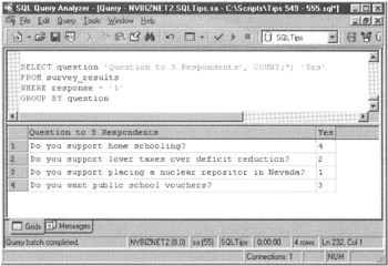
Figure 554.1: Grouped query results from the merged survey questions and responses working table

SELECT question 'Question to 5 Respondents', COUNT(*) 'Yes'
FROM survey_results
WHERE response = '1'
GROUP BY question

Using Views to Display a Hierarchy of Aggregation Levels

Most businesses are organized as hierarchies in which the span of responsibility and control increases as you move up the chain of command from worker to chief executive officer. At each level within the hierarchy, managers need summary reports to see how well their subordinates are doing. For example, in a sales organization, individual sales are grouped under the salesperson that made the sale. The department manager can then compare the effectiveness of one salesperson to another based on the total sales for each. Next, sales are grouped by department within region, so the regional vice president for sales can get a feel for how well his or her department managers are doing. Finally, regional sales are grouped together to give the company CEO the total sales information he or she must have to report on the company's overall sales growth (or lack thereof) to the board of directors and shareholders.

To build this hierarchy of summary information, you can use a sequence of SELECT statements and views to aggregate totals at each level of the hierarchy. As you work your way up the hierarchy of summary reports, each view is based on the summary of views from the previous step within the hierarchy. For example, you might create the following views to summarize company sales data by employee, department, and region:

CREATE VIEW vw_salesrep_sales (region, department,
 salesprep_ID, total_sales)
AS SELECT region, department, salesrep_ID SUM(amount)
FROM sales
GROUP BY region, department, salesrep_ID

CREATE VIEW vw_department_sales (region, department,
 total_sales
AS SELECT region, department, SUM(total_sales)
FROM vw_salesrep_sales
GROUP BY region, department

CREATE VIEW vw_regional_sales (region, total_sales)
AS SELECT region, SUM(total_sales)
FROM vw_department_sales
GROUP BY region

To generate a summary reports, execute SELECT statements based on the preceding views as shown here:

 SELECT * FROM vw_salesrep_sales
 SELECT * FROM vw_department_sales
 SELECT * FROM vw_region_sales

 SELECT SUM (total_sales)
 FROM vw_regional_sales

When run as a statement batch, executing these SELECT statements on views will likely run faster than executing the four queries directly on the base (SALES) table. If you query the SALES table without a VIEW, the DBMS must scan all the rows in the SALES table repeatedly (once for each query). By using views, the DBMS need only scan the SALES table once. Thereafter, the DBMS scans the virtual (either in memory or in disk cached) table created when the DBMS materialized the view at the preceding level within the hierarchy.

Understanding the MS SQL Server TOP n Operator

When querying a table, you sometimes want the DBMS to return only a certain number of rows. Suppose, for example, that you have 50 salespeople working for you. You might want a list of the top three salespeople by total sales so you can single them out for praise. Or, if you must cut your staff by 10 percent, you will want a list of the five salespeople with the least total sales so you can keep the 45 best producers. The MS-SQL Server TOP operator will scan the output from a query (or subquery) and return the first n rows it finds.

For example, to get a list of the three highest TOTAL_SALES values in the EMPLOYEES table within an MS-SQL Server database you could write a query similar to:

SELECT DISTINCT TOP 3 total_sales
FROM employees
ORDER BY total_sales DESC

The ORDER BY clause instructs the DBMS to build a virtual (in-memory) table of TOTAL_SALES values arranged in descending order. After building the virtual table, the DBMS applies the DISTINCT clause and eliminates any duplicate rows from the interim table. Finally, the TOP operator has the DBMS return only the first n, in this case three rows from the virtual table as the query's results set.

If you omit the DISTINCT clause, the results set will have less than three unique values when there is a tie between two or more of the top three values within the list. Suppose, for example, that the EMPLOYEES table had the following values within the TOTAL_SALES column:

 TOTAL_SALES
 -----------
 115,000.00
 100,000.00
 105,000.00
 100,000.00
 85,000.00
 85,000.00
 105,000.00
 65,000.00
 95,000.00
 95,000.00

The query (with the DISTINCT clause) in this example will return the three values: 115,000.00, 105,000.00, and 100,000.00. However, if you rewrote the query without the DISTINCT clause as

 SELECT TOP 3 total_sales
 FROM employees
 ORDER BY total_sales DESC

the results set would be 115,000.00, 105,000.00, and 105,000.00. Note that you still get three rows of results. However, the results set has only two unique TOTAL_SALES values due to the tie at 105,000.00.

Transact-SQL has no BOTTOM operator you can use to tell the DBMS to return the BOTTOM n rows of query results. However, you can use the TOP operator to retrieve the bottom or last n rows of query results just as you had TOP return the top or first n rows. If you want to get a list of the bottom three TOTAL_SALES values (versus the top three), simply reverse the query's sort order from DESC to ASC as shown here:

 SELECT DISTINCT TOP 3 total_sales
 FROM employees
 ORDER BY total_sales ASC

Once again the DBMS will build a virtual (in-memory) table of TOTAL_SALES values. Only this time, the ORDER BY clause instructs the DBMS to build the virtual table with the values arranged in ascending order . After building the virtual table of TOTAL_SALES values, the DBMS eliminates any duplicate rows (as instructed by the DISTINCT clause). Then, the TOP operator has the DBMS return the first three rows from the virtual table as the query's results set.

Because the ORDER BY clause has the DBMS sort the virtual table from lowest to highest value, the results set will have the three lowest TOTAL_SALES values in the first (that is, the top) three rows within the virtual table. As such, the query (with the ascending sort) in this example will return the values: 65,000.00, 85,000.00, and 95,000.00.

To list the names and TOTAL_SALES figures for your top n (or bottom n) salespeople, use a SELECT statement with the TOP operator as a subquery to build the list of top TOTAL_SALES values. For example, the following query will display the names and total sales amounts (in descending order by TOTAL_SALES value) of the employees with TOTAL_SALES equal to one of the top three values in the TOTAL_SALES column:

SELECT first_name, last_name, total_sales
FROM employees
WHERE total_sales IN (SELECT DISTINCT TOP 3 total_sales
 FROM employees
 ORDER BY total_sales DESC)

By the way, Transact-SQL also lets you express the number of rows you want the DBMS to return as a percentage of the total number or rows that satisfy the query's search conditions. Therefore, in this example in which the EMPLOYEES table has 10 rows, you could limit the results set from the following query to five rows by setting the TOP operator to 50 percent:

 SELECT TOP 50 percent total_sales
 FROM employees
 ORDER BY total_sales DESC

If you apply the DISTINCT clause by writing the query as follows, the DBMS will return only three rows, because the EMPLOYEES table in this tip's example has only six unique values within the TOTAL_SALES column:

 SELECT DISTINCT TOP 50 percent total_sales
 FROM employees
 ORDER BY total_sales DESC

(The DBMS returns three rows, because three represents 50 percent of the six unique rows the query leaves in the interim [virtual] table it generates prior to returning the final results set.)

Constructing a Top n or Bottom n Query Within a DBMS Without a TOP n Operator

In the preceding tip "Understanding the MS-SQL Server TOP n Operator," you learned how to use the Transact-SQL TOP operator to have the MS-SQL Server return the first n results that satisfy a query's search conditions. Unfortunately, some DBMS products do not have a TOP operator. If your DBMS is one of these, all is not lost. You can limit the number of rows within a results set by using either a grouped query or a SELECT statement with a correlated subquery.

Suppose for example that you had the following data within an EMPLOYEES table and wanted the retrieve the rows with the top three TOTAL_SALES values:

 FIRST_NAME LAST_NAME TOTAL_SALES
 ---------- --------- -----------
 Konrad Kernin 115,000.00
 Joseph King 100,000.00
 Sally Hardy 105,000.00
 Robert Fields 100,000.00
 Walter Berry 85,000.00
 Susan Mathau 85,000.00
 Karen Berry 105,000.00
 Kregg King 65,000.00
 Kris Smith 95,000.00
 Debbie Jones 95,000.00

To construct a grouped query that will return the top n TOTAL_SALES values, you must apply a bit of set logic. The idea is to take each value within the TOTALS_SALES column and build a set (or group) of other TOTAL_SALES values that are greater than or equal to it. The lowest TOTAL_SALES value within the sets (or groups) that have n or fewer unique members are the ones you want the DBMS to return. In this example, you want the DBMS to return the lowest TOTAL_SALES value from sets that have at most three unique members. (If you wanted the top five TOTAL_SALES values, you'd have the DBMS to return the SETS with at most five unique members, and so on.)

Therefore, you write the grouped query that will return the top three TOTAL_SALES values as follows:

 SELECT MIN(e1.total_sales) 'Top Three TOTAL_SALES'
 FROM employees AS e1, employees AS e2
 WHERE e1.total_sales >= e2.total_sales
 GROUP BY e2.total_sales
 HAVING COUNT(DISTINCT e1.total_sales) <= 3

The query's HAVING clause tells the DBMS to keep within the interim (virtual) table only those sets of TOTAL_SALES values that have three or less unique members. Then, the MIN() aggregate in the query's SELECT clause tells the DBMS to return the minimum TOTAL_SALES value from each of the remaining sets (with three, two, or one unique values).

To return the bottom three (that is the three lowest) TOTAL_SALES values, simply change the comparison operator within the HAVING clause from "<=" to ">" as follows:

 SELECT MIN(e1.total_sales) 'Bottom Three TOTAL_SALES'
 FROM employees AS e1, employees AS e2
 WHERE e1.total_sales >= e2.total_sales
 GROUP BY e2.total_sales
 HAVING COUNT(DISTINCT e1.total_sales) > 3

If you want the query to return something other than the top (or bottom) three values, change the "3" within the HAVING clause to the number of rows you want the query to return.

Rather than write the SELECT statement as a grouped query, you can have the DBMS return the top (or bottom) n values using a SELECT statement that has a correlated subquery that builds and eliminates the sets of TOTAL_SALES values with more than n unique members. For example, to have the DBMS return the top three TOTAL_SALES values from the employees table, you can write the query as:

 SELECT DISTINCT e1.total_sales 'Top Three TOTAL_SALES'
 FROM employees AS el
 WHERE 3 < (SELECT COUNT(*) FROM employees AS e2
 WHERE e1.total_sales > e2.total_sales)

The DISTINCT clause eliminates duplicate TOTAL_SALES values from the results set in case of a tie among two or more of the top values within the TOTAL_SALES column in the EMPLOYEES table.

To display the list of the bottom (that is, the lowest) n values within a column, simply change the comparison operator within the correlated subquery's WHERE clause from less than (<) to greater than (>) as shown here:

SELECT DISTINCT e1.total_sales 'Bottom Three TOTAL_SALES'
FROM employees AS el
WHERE 3 < (SELECT COUNT(*) FROM employees AS e2
 WHERE e1.total_sales < e2.total_sales)

If you want to list the names as well as the TOTAL_SALES figures for your top n (or bottom n) salespeople, add the columns whose values you want to display to the SELECT clause as shown in the following query:

SELECT first_name, last_name, total_sales
FROM employees AS e1
WHERE 3 < (SELECT COUNT(*) FROM employees AS e2
 WHERE e1.total_sales > e2.total_sales)
ORDER BY total_sales DESC

It probably goes without saying, however there is nothing magic about the "3" used in the preceding examples. If you wanted to list the top (or bottom) five salespeople by TOTAL_SALES, you would simply replace the "3" within the WHERE clause of each query with "5."

Using a SELECT Statement with a Scalar Subquery to Display Running Totals

While SQL is an excellent language for data storage and retrieval, it is not much of a report writer. SQL can compute the total, average, minimum, or maximum value for a column easily. However, SQL's ability to provide totals for columns of numbers within groups of rows is limited. Whereas a report writer can make multiple passes through report data to provide descriptive statistics for groups (and groups of groups) while still providing the detail rows, SQL's totaling ability (provided by GROUP BY clause) forces you to give up detail rows if you want group totals.

For example, a report writer can provide total sales by salesperson, grand total sales for all salespeople, along with the rows of data that provide information on each sale. If you want SQL to provide total sales by salesperson, you must execute a grouped query such as the following and give up the detailed sales information:

 SELECT salesrep_ID, SUM(amount_invoiced) 'Total Sales'
 FROM sales
 GROUP BY salesrep_ID
 ORDER BY salesrep_ID

Although you could have reported both totals and detail by computing the total sales with a subquery within the main query's SELECT clause (as shown next), seeing the same total sales figure repeatedly down one column of the report can be confusing:

 SELECT *, (SELECT SUM(amount_invoiced)
 FROM sales AS s2
 WHERE s2.salesrep_ID = s1.salesrep_ID) AS
 'Total Sales'
 FROM sales AS s1
 ORDER BY salesrep_ID, invoice_date

Whereas displaying a grand total on every detail line is less than desirable, using a scalar subquery to provide a running total can sometimes increase a report's usefulness. Suppose, for example that you have a table with check (or withdrawal) and deposit transactions. If the TRANS_AMOUNT column contains a negative value for withdrawals and positive value for deposits, you can use the following query to list the transactions, as well as the running total of deposits less withdrawals:

SELECT t1.trans_date, trans_type, trans_amount AS 'Amount'
 (SELECT SUM(t2.trans_amount)
 FROM transactions AS t2
 WHERE t2.trans_date <= t1.trans_date) AS
 'Net (Deposits - Checks)'
 FROM transactions AS t1
 ORDER BY trans_date

Of course, to be truly useful, you will want to execute the preceding query within a stored procedure or a statement batch in which you have the account counter within a variable such as @ACCT_NO and the account's beginning balance would be @BEGIN_BAL. You could then add the beginning balance to the net transaction amount to display a running account balance and limit the query to showing only a particular account's transactions (versus all checks and deposits within the TRANSACTIONS table):

SELECT t1.trans_date, trans_type, trans_amount AS 'Amount'
 (SELECT SUM(t2.trans_amount)
 FROM transactions AS t2
 WHERE t2.trans_date <= t1.trans_date
 AND t2.acct_number = @acct_no) + @begin_bal)
 AS 'Account Balance'
FROM transactions AS t1
WHERE t1.acct_number = @acct_no
ORDER BY trans_date

Using an EXCEPT Predicate to Determine the Difference Between Two Tables

The set difference operator, EXCEPT, lets you determine the rows in TABLE_A that are not also in TABLE_B. Thus, if you load the list of all students into TABLE_A and the list of students that have completed their core requirements into TABLE_B, you can use the following statement to display all students except those that have completed their core requirements:

 SELECT * FROM table_a
 EXCEPT
 SELECT * FROM table_b

Note that the EXCEPT operator eliminates all duplicates from the first query (SELECT * FROM TABLE_A) before comparing its results set with that of the second query (SELECT * FROM TABLE_B). Thus, the results set from an EXCEPT query will never contain any duplicate rows.

Although the query in this example assumed they were, the EXCEPT statement does not require that TABLE_A and TABLE_B be union compatible. As you learned previously, two tables are union-compatible if both have the same number of columns and if the data type of each column in one table is the same as the data type of its corresponding column (by ordinal position) in the other table.

Because the EXCEPT operator returns all rows in the first results set that do not appear in the second, you can use EXCEPT with two dissimilar (that is, non union-compatible) tables by simply listing the columns from each table the operator is to compare. Thus, to list all customers that are not also employees, you might write the following query:

 SELECT first_name, last_name, phone_number FROM customers
 EXCEPT
 SELECT first_name, last_name, phone_number FROM employees

Unfortunately, many DBMS products have not yet implemented the EXCEPT operator. As such, you may have to use a LEFT OUTER JOIN instead. Suppose, for example, that you buy a prospect list and want to eliminate your current customers before turning the list over to your sales force. You could load the prospect list data into a table named PROSPECTS and use the following LEFT OUTER JOIN to generate a list of PROSPECTS that are not also CUSTOMERS:

 SELECT DISTINCT prospects.*
 FROM (prospects LEFT OUTER JOIN customers
 ON prospects.phone_number = customers.phone_number)
 WHERE customers.phone_number IS NULL

The preceding query assumes that PHONE_NUMBER is either a PRIMARY KEY or a column with values that uniquely identify both individual prospects and customers.

Note 

Some DBMS products implement the EXCEPT operator under a different name. Oracle for example, uses MINUS. Therefore, before substituting a less efficient LEFT OUTER JOIN for EXCEPT, check your DBMS documentation to see if EXCEPT is implemented.

Using the EXISTS Predicate to Generate the Intersection Between Two Tables

When you want to know which rows two tables have in common, use the INTERSECTION operator. Whereas the EXCEPT operator (which you learned about in Tip 559 " Using an EXCEPT Predicate to Determine the Difference Between Two Tables") returns the rows within the first results set that are not within the second, the INTERSECT operator returns only those rows that appear in both results sets. Thus, if your company sells insurance and you want a list of customers that purchase both life and auto insurance from you, you might use a query similar to the following:

 SELECT cust_ID, first_name, last_name, phone_number
 FROM life_cust_list
 INTERSECT
 SELECT cust_ID, first_name, last_name, phone_number
 FROM auto_cust_list

As was the case with the EXCEPT operator, the two tables you use with the INTERSECT operator need not be union-compatible. However, the component queries before and after the INTERSECT keyword must return the same number of columns and corresponding columns must be of the compatible data types. In addition to returning only rows that appear in both results sets, the INTERSECT operator also eliminates all duplicates.

Only a few DBMS products have implemented the INTERSECT operator at present. However, you can use a SELECT statement with an EXISTS predicate to generate the intersection of two tables instead. For example, if you want to generate the list of students that are both on the Dean's List and the football team, you might generate the following query:

 SELECT DISTINCT student_id, first_name, last_name, GPA
 FROM students
 WHERE EXISTS (SELECT * FROM football_team
 WHERE students.student_ID =
 football_team.student_ID)

You can also write the same query using an INNER JOIN as:

SELECT DISTINCT student_id, first_name, last_name, GPA
FROM students INNER JOIN football_team
 ON students.student_ID = football_team,student_ID