Understanding SQL Basics and Creating Database Files

Understanding the Definition of a Database

Many people use the term database to mean any collection of data items. Working as a consultant, I've been called onsite to repair a database, only to find that the client was referring to a customer list in a Corel WordPerfect document that appeared "corrupted" because someone had changed the document's margins. Microsoft and Lotus have also blurred the lines between application data and a database by referring to "database" queries in help screens about searching the information stored in the cells that make up their competing spreadsheet products.

As the name implies, a database contains data. The data is organized into records that describe a physical or conceptual object. Related database records are grouped together into tables. A customer record, for example, could consist of data items, or attributes, such as name, customer number, address, phone number, credit rating, birthday, anniversary, and so on. In short, a customer record is any group of attributes or characteristics that uniquely identify a person (or other business), making it possible to market the customer for new business or to deliver goods or services. A customer table, then, is a collection of customer records. Similarly, if a business wants to track its inventory (or collection of goods for sale), it would create an inventory table consisting of inventory records. Each inventory record would contain multiple attributes that uniquely describe each item in the inventory. These attributes might include item number, description, cost, date manufactured or purchased, and so on.

While a flat file (which we'll discuss in Tip 2, "Understanding Flat Files,") contains only data, a database contains both data and metadata. Metadata is a description of:

• The fields in each record (or columns in a table)
• The location, name, and number of records in each table
• The indexes used to find records in tables
• The value constraints that define the range of values that can be assigned to individual record attributes (or fields)
• The key constraints that define what records can be added to a table and that limit the way in which records can be removed; also the relationship between records in different database tables

While the data in a database is organized into related records within multiple tables, the metadata for a database is placed in a single table called the data dictionary.

In short, a database is defined as a self-describing collection of records organized into tables. The database is self-describing because it contains metadata in a data dictionary table that describes the fields (or attributes) in each record (or table row) and the structure that groups related records into tables.

Understanding Flat Files

Flat files are collections of data records. When looking at the contents of a flat file, you will not find any information (metadata) that describes the data in the file. Instead, you will see row after row of data such as the following:

 010000BREAKFAST JUICES F00.000000
 010200TREE TOP APPLE JUICE 120ZF01.100422
 010400WELCHES GRAPE JUICE 12OZF00.850198
 010600MINUTE MAID LEMONADE 12OZF00.850083
 010800MINUTE MAID PINK LEMONADE 12OZF00.890099
 011000MINUTE MAID ORANGE JUICE 12OZF01.260704
 011400MINUTE MAID FRUIT PUNCH 120ZF00.820142
 011600CAMPBELLS CAN TOMATO JUICE 46OZG01.200030
 020000FAMOUS BRAND CEREALS G01.200000
 020200GENERAL MILLS CHEERIOS 15OZG03.010050

Looking at the flat file listing, you can see that the file contains only data. Spaces are used to separate one field from another and each non-blank line is a record. Each application program reading the data file must "know" the number of characters in each "field" and what the data means. As such, programs must have lines of code that read the first 6 characters on a line as an item number and the next 32 characters as a description, followed by a 1-character department indicator, followed by a 5-character sales price, and ending with a 4-digit average count delivered each week. COBOL programs using flat files had a "File Description" that described the layout of each line (or record) to be read. Modern programming languages such as Pascal, C, and Visual Basic let you read each line of the flat file as a text string that you can then divide into parts and assign to variables whose meanings you define elsewhere in the application. The important thing to understand is that every program using a flat file must have its own description of the file's data. Conversely, the description of the records in a database table is stored in the data dictionary within the database itself. When you change the layout of the records in a flat file (by inserting a five-character item cost field after the sales price, for example), you must change all of the programs that read data from the flat file. If you change the fields in a database record, you need change only the data dictionary. Programs reading database records need not be changed and recompiled.

Another difference between flat files and a database is the way in which files are managed. While a database file (which consists of one or more tables) is managed by the database management system (DBMS), flat files are under the control of the computer operating system's file management system. A file management system, unlike a DBMS, does not keep track of the type of data a file contains. As such, the file system handles word-processing documents, spreadsheets, and graphic images the same way—it keeps track of each file's location and size. Every program that works with a flat file must have lines of code that define the type of data inside the file and how to manipulate it. When developing applications that work with database tables, the programmer needs to specify only what is to be done with the data. While the programmer working with a flat file must know how and where the data is stored, the database programmer is freed from having to know these details. Instead, of having to program how the file manager is to read, add, or remove records, the database programmer needs to specify only which actions the DBMS is to take. The DBMS takes care of the physical manipulation of the data.

Unfortunately, each operating system (DOS, Windows, Unix, and OS2, to name a few) has a different set of commands that you must use to access files. As a result, programs written to use flat file data are not transportable from one operating system to another since the data-manipulation code is often specific to a particular hardware platform. Conversely, programs written to manipulate database data are transportable because the applications make use of high-level read, write, and delete commands sent to the DBMS, which performs the specific steps necessary to carry them out. A delete command sent to the DBMS by an application running on a Unix system is the same delete command a DBMS running on Windows NT expects to see. The physical steps taken to carry out the command differ, but these steps are handled by the DBMS and hidden from the application program.

Thus, the major differences between a flat file and a database are that the flat file is managed by the operating system's file management system and contains no description of its contents. As a result, application programs working with a flat file must include a definition of the flat file record layout, code that specifies the activity (read, write, delete) to be performed, and low-level operating system-specific commands to carry out the program's intent. A database, on the other hand, is managed by the DBMS that handles the low-level commands that manipulate the database file data. In short, programs that work with flat files define the data and the commands that specify what to do and how to do it. Programs that work with a database specify only what is to be done and leave the details of how it is to be done to the DBMS.

Understanding the Hierarchical Database Model

A hierarchical database model consists of data arranged into a structure that looks a lot like a family tree or company organizational chart. If you need to manage data that lends itself to being represented as parent/child relationships, you can make use of the hierarchical database model. Suppose, for example, that you have a home food delivery service and need to know how much of each grocery item you have to purchase in order to fill your customer orders for a particular delivery date. You might design your database using the hierarchical model similar to that shown in Figure 3.1.

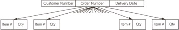
Figure 3.1: Hierarchical database model with ORDER/ITEM parent/child relationships

In a hierarchical database, each parent record can have multiple child records; however, each child must have one and only one parent. The hierarchical database for the home food delivery service orders consists of two tables: ORDER (with fields: CUSTOMER NUMBER, ORDER NUMBER, DELIVERY DATE) and ITEM (with fields: ITEM NUMBER, QUANTITY). Each ORDER (parent) record has multiple ITEM (child) records. Conversely, each ITEM (child) record has one parent—the ORDER record for the date on which the item is to be delivered. As such, the database conforms to the hierarchical database model.

To work with data in the database, a program must navigate its hierarchical structure by:

• Finding a particular parent or child record (that is, find an ORDER record by date, or find an ITEM by ITEM NUMBER)
• Moving "down," from parent to child (from ORDER to ITEM)
• Moving "up," from child to parent (from ITEM to ORDER)
• Moving "sideways," from child to child (from ITEM to ITEM) or parent to parent (from ORDER to ORDER)

Thus, to generate a purchase order for the items needed to fill all customer orders for a particular date, the program would:

1. Find an ORDER record for a particular date.
2. Move down to the first ITEM (child) record and add the amount in the quantity field to the count of that item number to be delivered. For example, if the first item were item number 10 with a quantity of 5, the program would add 5 to the count of item 10s to be delivered on the delivery date.
3. Move sideways to the next ITEM (child) record and add the amount in its quantity field to the count of that item number to be delivered. For example, if the next ITEM (child) record for this order were 15 with a quantity of 4, the program would add 4 to the count of item 15s to be delivered on the delivery date.
4. Repeat Step 3 until there are no more child records.
5. Move up to the ORDER (parent) record.
6. Move sideways to the next ORDER (parent) record. If the ORDER record has a delivery equal to the one for which the program is generating the purchase order, continue at Step 2. If there are no more ORDER records, or if the delivery date in the ORDER record is not equal to the date for which the program is generating a purchase order, continue at Step 7.
7. Output the purchase order by printing the item number and quantity to be delivered for each of the items with a nonzero delivery count.

The main advantages of the hierarchical database are:

• Performance. Navigating among the records in a hierarchical database is very fast because the parent/child relationships are implemented with pointers from one data record to another. The same is true for the sideways relationships from child to child and parent to parent. Thus, after finding the first record, the program does not have to search an index (or do a table scan) to find the next record. Instead, the application needs only to follow one of the multiple child record pointers, the single sibling record pointer, or the single parent record pointer to get to the "next" record.
• Ease of understanding. The organization of the database parallels a corporate organization chart or family tree. As such, it has a familiar "feel" to even nonprogrammers. Moreover, it easily depicts relationships where A is a part of B (as was the case with the order database we discussed, where each item was a part of an order).

The main disadvantage of the hierarchical database is its rigid structure. If you want to add a field to a table, the database management system must create a new table for the larger records. Unlike an SQL database, the hierarchical model has no ALTER TABLE command. Moreover, if you want to add a new relationship, you will have to build a new and possibly redundant database structure. Suppose, for example, that you want to track the orders for both a customer and all of the customers for a salesperson; you would have to create a hierarchical structure similar to that shown in Figure 3.2.

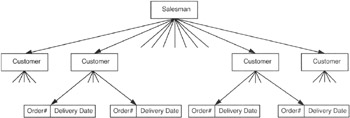
Figure 3.2: Hierarchical database model with SALESMAN, CUSTOMER, and ORDER relationships

If you just rebuild the ORDER records to include the salesman and leave the database structure as shown in Figure 3.1, your application would have to visit each and every ORDER record to find all of the customers for a particular salesman or all of the orders for a particular customer. Remember, each record in the hierarchical model has only one sibling pointer for use in moving laterally through the database. In our example database, ORDER records are linked by delivery date to make it easy to find all orders for a particular delivery date. Without knowing the date range in which a particular customer placed his or her order(s), you have to visit every ORDER record to see if it belongs to a specific customer. If you decide to restructure the original database instead of creating the redundant ORDER table, you increase the time it takes to find all of the orders for a particular delivery date. In the restructured database, moving laterally at the ORDER record level of the tree gives you only the ORDER records for a particular customer, since ORDER records are now children of a CUSTOMER record parent.

Understanding the Network Database Model

The network database model extends the hierarchiear model by allowing a record to participate in multiple parent/child relationships. In order to be helpful, a database model must be able to represent data relationships in a database to mirror those we see in the real world. One of the shortcomings of the hierarchical database model was that a child record could have one and only one parent. As a result, if you needed to model a more complex relationship, you had to create redundant tables. For example, suppose you were implementing an order-processing system. You would need at least three parent/child relationships for the same ORDER record, as shown in Figure 4.1.

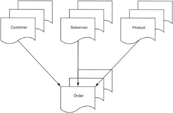
Figure 4.1: Database requiring multiple parent/child relationships

You need to be able to print out an invoice for the orders placed by your customers, so you need to know which orders belong to which customer. The salesmen need to be paid commissions, so you need to know which orders each of them generated. Finally, the production department needs to know which parts are allocated to which orders so that it can assemble the orders and maintain an inventory of products to fill future orders.

If you were to use the hierarchical model, you would have to produce three ORDER tables, one for each of the three parents of each ORDER record. Redundant tables take up additional disk space and increase the processing time required to complete a transaction. Consider what happens if you need to enter an order into a hierarchical database that has redundant ORDER tables. In the current example with three parent/child relationships to ORDER records, the program must insert each new ORDER record into three tables. Conversely, if you had a database that allowed a record to have more than one parent, you would have to do only a single insert.

In addition to allowing child records to have multiple parents, the network database model introduced the concepts of "sets" to the database processing. Using the network database model, you could structure the order-processing database relationships shown in Figure 4.1 as shown in Figure 4.2.

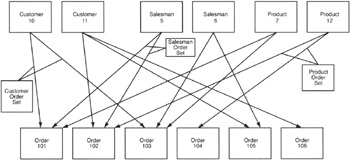
Figure 4.2: A database for an order-processing system based on the network database model

Look at Figure 4.2, and you will see that ORDER 101 and ORDER 103 belong to (or are the children of) CUSTOMER 10. Meanwhile, ORDER 102, ORDER 105, and ORDER 106 belong to CUSTOMER 11. As mentioned previously, the network database model applies set concepts to database processing. Refer again to Figure 4.2, and note that the orders that belong to CUSTOMER 10 (ORDER 101 and ORDER 103) are defined as the Customer Order Set for CUSTOMER 10. Similarly, ORDERS 102, 105, and 106 are the Customer Order Set for CUSTOMER 11. Moving next to the SALESMEN records, you can see that SALESMAN 5 was responsible for ORDER 101 and ORDER 102. Meanwhile SALESMAN 6 was responsible for ORDER 103 and ORDER 105. Thus, the Salesman Order Set for SALESMAN 5 consists of ORDERS 101 and 102, and the Salesman Order Set for SALESMAN 6 includes ORDERS 103 and 105. Finally, moving on to the PRODUCTS table, you can see that that PRODUCT 7 is on ORDER 101 and ORDER 103. PRODUCT 12, meanwhile, is on ORDER 102 and ORDER 104. As such, the Product Order Set for PRODUCT 7 consists of ORDERS 102 and 104; while the Product Order Set for PRODUCT 12 includes ORDERS 102 and 104.

Note 

The company will, of course, have more customers, salesmen, products, and orders than those shown in Figure 4.2. The additional customers, salesmen, and products would be represented as additional parent records in their respective tables. Meanwhile, each of the additional ORDER (child) records in the ORDER table would be an element in each of the three record sets (Customer Order Set, Salesman Order Set, and Product Order Set).

To retrieve the data in the database, a program must navigate the hierarchical structure by:

• Finding a parent or child record (finding a SALESMAN by number, for example)
• Moving "down," from parent to the first child in a particular set (from SALESMAN to ORDER, for example)
• Moving "sideways," from child to child in the same set (from ORDER to ORDER, for example), or from parent to parent (from CUSTOMER to CUSTOMER, SALESMAN to SALESMAN, or PRODUCT to PRODUCT)
• Moving "up," from child to parent in the same set, or from child to parent in another set (from ORDER to SALESMAN or from ORDER to PRODUCT or from ORDER to CUSTOMER)

Thus, getting information out of a network database is similar to getting data out of the hierarchical database-the program moves rapidly from record to record using a pointer to the "next" record. In the network database, however, the programmer must specify not only the direction of the navigation (down, sideways, or up), but also the set (or relationship) when traveling up (from child record to parent) and sideways (from child to child in the same set).

Because the network database model allows a child record to have multiple parent records, an application program can use a single table to report on multiple relationships. Using the order-processing database example, a report program can use the ORDER table to report which orders include a particular product, which customers bought the product, and which salesmen sold it by performing the following steps:

1. Find a PRODUCT record by description or product number.
2. Move down to the first ORDER record (which contains the product) in the Product Order Set.
3. Find the CUSTOMER that ordered the product (placed the order) by moving up to the parent of the Customer Order Set.
4. Return to the child ORDER record by moving back down the link ascended in Step 3.
5. Find the SALESMAN that sold the product (got the customer to place the order) by moving up to the parent of the Salesman Order Set.
6. Return to the child ORDER record by moving back down the link ascended in Step 5.
7. Move sideways to the next ORDER (child) record in the Product Order Set. If there is another child record, continue at Step 2.

The main advantages of the hierarchical database are:

• Performance. Although the network database model is more complex than the hierarchical database model (with several additional pointers in each record), its overall performance is comparable to that of its predecessor. While the DBMS has to spend more time maintaining record pointers in the network model, it spends less time inserting and removing records due to the elimination of redundant tables.
• Ability to represent complex relationships. By allowing more than one parent/child link in each record, the network database model lets you extract data based on multiple relationships using a single table. While we explored using the network database to get a list of all customers that purchased a product and all salesmen that sold the product, you could also get a list of the orders placed by one or all of the customers and a list of sales made by one salesman or the entire sales force using the same network database structure and the same set of tables.

Unfortunately, the network database model, like its hierarchical rival, has the disadvantage of being inflexible. If you want to add a field to a table, the DBMS must create a new table for the larger records. Like the hierarchical model (and, again, unlike an SQL relational database), the network model has no ALTER TABLE command. Moreover, rebuilding a table to accommodate a change in a record's attributes or adding a new table to represent another relationship requires that a majority of the network database's record links be recalculated and updated-this translates into the database being inaccessible for extended periods of time to make even a minor change to a single table's fields.

Understanding the Relational Database Model

While the relational database model did not appear in commercial products until the 1980s, Dr. Edgar F. Codd of IBM defined the relational database in 1970. The relational model simplifies database structures by eliminating the explicit parent/child relationship pointers. In a relational database, all data is organized into tables. The hierarchical and network database records are represented by table rows, record fields (or attributes) are represented as table columns, and pointers to parent and child records are eliminated.

A relational database can still represent parent/child relationships, it just does it based on data values in its tables. For example, you can represent the complex Network database model data shown in Figure 4.2 of Tip 4 with the tables shown in Figure 5.1.

Customer Table
CUST_NO	LAST_NAME	FIRST_NAME
10	FIELDS	SALLY
11	CLEAVER	WARD

Salesman Table
SALESMAN_NO	LAST_NAME	FIRST_NAME
5	KING	KAREN
6	HARDY	ROBERT

Product Table
PRODUCT_NO	DESCRIPTION	SALES_PRICE	INV_COUNT
7	100 WATT SPEAKER	75.00	25
8	DVD PLAYER	90.00	15
9	AMPLIFIER	450.00	305
10	RECEIVER	750.00	25
11	REMOTE CONTROL	25.00	15
12	50 DVD PACK	500.00	25

Order Table
ORDER NO	DEL DATE	PRODUCT_NO	SALESMAN_NO	CUST_NO
101	01/15/2000	7	5	10
102	01/22/2000	12	5	11
103	03/15/2000	7	6	10
104	04/05/2000	12	7	12
105	07/05/2000	9	6	11
106	08/09/2000	7	8	11

Figure 5.1: ORDER_ TABLE with relationships to three other tables

In place of pointers, the relational database model uses common columns to establish the relationship between tables. For example, looking at Figure 5.1, you will see that the CUSTOMER, SALESMAN, and PRODUCT tables are not related because they have no columns in common. However, the ORDER table is related to the CUSTOMER table by the CUSTOMER_NO column. As such, an ORDER table row is related to a CUSTOMER table row where the CUSTOMER_NO column has the same value in both tables. Figure 5.1 shows CUSTOMER 10 owns ORDER 101 and ORDER 103 since the CUST_NO column for these two ORDER rows is equal to the CUSTOMER_NO column in the CUSTOMER table. The SALESMAN and PRODUCT tables are related to the ORDER table in the same manner. The SALESMAN table is related to the ORDER table by the common SALESMAN_NO column, and the PRODUCT table is related to the ORDER table by the PRODUCT_NO column.

As you may have noticed from the discussion of the hierarchical model in Tip 3, "Understanding the Hierarchical Database Model," and the network model in Tip 4, applications written to extract data from either of these models had the database structures "hard-coded" into them. To navigate the records in the network model, for example, the programmer had to know what pointers were available and what type of data existed at each level of the database tree structure. Knowing the names of the pointers let the programmer move up, down, or across the database tree; knowing what data was available at each level of the tree told the programmer the direction in which to move. Because record relationships based on pointers are hard-coded into the application, adding a new level to the tree structure requires that you change the application program's logic. Even just adding a new attribute to a network database record changes the location of the pointer within the record changes. As a result, any changes to a database record require that the application programs accessing the database be recompiled or rewritten.

When working with a relational database, you can add tables and add columns to tables to create new relationships to the new tables without recompiling existing applications. The only time you need to recompile an application is if you delete or change a column used by that program. Thus, if you want to relate an entry in the SALESMAN table to a customer (in the CUSTOMER table), you need only add a SALESMAN_NO column to the CUSTOMER table.

Understanding Codd s 12 Rule Relational Database Definition

Dr. Edgar F. Codd published the first theoretical model of a relational database in an article entitled "A Relational Model of Data for Large Shared Data Banks" in the Communications of the ACM in 1970. The relational model was theoretical at the time because all commercially available database management systems were based on either the hierarchical or the network database models. Although Dr. Codd worked for IBM, it was Oracle that brought the first database based on the relational model to market in 1980—10 years later! While Dr. Codd's 12 rules are the semi-official definition of a relational database, and while many commercial databases call themselves relational today, no relational database follows all 12 rules.

Codd's 12 rules to define a relational database are:

1. The Information Rule. All information in a relational database must be represented in one and only one way, by values in columns within rows of tables. SQL satisfies this rule.
2. The Guaranteed Access Rule. Each and every datum (or individual column value in a row) must be logically addressable by specifying the name of the table, primary key value, and column name. When addressing a data item, the name of the table identifies which database table contains the item, the column identifies a specific item in a row of the named table, and the primary key identifies a single row within a table. SQL follows this rule for tables with primary keys. However, SQL does not require that a table have a key.
3. Systematic Treatment of Null Values. The relational database management system must be able to represent missing and inapplicable information in a systematic way that is independent of data type, different than that used to show empty character strings or a strings of blank characters, and distinct from zero or any other number. SQL uses NULL to represent both missing and inapplicable information—as you will learn later, NULL is not zero, nor is it an empty string.
4. Dynamic Online Catalog Based on the Relational Model. The database catalog (or description) is represented in the same manner as ordinary data (using tables), so authorized users can use the same relational language to work with the online catalog and regular data. SQL does this through system tables whose columns describe the structure of the database.
5. Comprehensive Data Sublanguage Rule. The system may support more than one language, but at least one language must have a well-defined syntax that is based on character strings and that can be used both interactively and within application programs. The language must support:
   • Data definitions
   • View definitions
   • Data manipulation (both update and retrieval)
   • Security
   • Integrity constraints
   • Transaction management operations (Begin, Commit, Rollback)

   SQL Data Manipulation Language (DML) (which can be used both interactively and in application programs) has statements that perform all of the required operations.

6. View Updating Rule. All views that are theoretically updateable must be updateable by the system. (Views are virtual tables that give users different "pictures" or representations of the database structure.) SQL does not fully satisfy this rule in that it limits updateable views to those based on queries on a single table without GROUP BY or HAVING clauses; it also has no aggregate functions, no calculated columns, and no SELECT DISTINCT clause. Moreover, the view must contain a key of the table, and any columns excluded from the view must be NULL-able in the base table.
7. High-Level Insert, Update, and Delete. The system must support multiple-row and table (set-at-a-time) Insert, Update, and Delete operations. SQL does this by treating rows as sets in Insert, Update, and Delete operations. Rule 7 is designed to exclude systems that support only row-at-a-time navigation and modification of the database, such as that required by the hierarchical and network database models. SQL fully satisfies this rule.
8. Physical Data Independence. Application programs and interactive database access methods don't have to change due to a change in the physical storage device or method used to retrieve data from that device. SQL does this well.
9. Logical Data Independence. Application programs and interactive database access methods don't have to change if tables are changed in a way that preserves the original table values. SQL satisfies this requirement—the results of queries and action taken by statements do not depend on the arrangement of columns in a row, the position of rows in a table, or the structure used to represent the table inside the computer system.
10. Integrity Independence. All integrity constraints specific to a particular relational database must be definable in the relational sub-language, be specified outside of the application programs, and stored in the database catalogue. SQL-92 has integrity independence.
11. Distribution Independence. Applications and end users should not be aware of whether the database data exists in a single location or whether it is replicated on and distributed among many computers on a network. Thus, the database language must be able to use the same commands to query and manipulate distributed data located on both local and remote computer systems. Distributed SQL database products are relatively new, so the jury is still out as to how well they will satisfy this criterion.
12. The Nonsubversion Rule. If the system provides a low-level (record-at-a-time) interface, the low-level statements cannot be used to bypass integrity rules and constraints expressed in the high-level (set-at-a-time) language. SQL-92 complies with this rule. Although one can write statements that affect individual table rows, the system will still enforce security and referential integrity rules.

Just as no SQL DBMS complies with all of the specifications in the SQL-92 standard, none of the commercially available relational databases follow all of Codd's 12 rules. Rather than comparing scorecards on the number of Codd's rules a relational database satisfies, companies normally select a particular database product based on performance, features, availability of development tools, and quality of vendor support. However, Codd's rules are important from a historical prospective, and they do help you decide whether a DBMS is based on the relational model.

Understanding Terms Used to Define an SQL Database

Tables

Every SQL database is based on the relational database model. As such, the individual data items in an SQL database are organized into tables. An SQL table (sometimes called a relation), consists of a two-dimensional array of rows and columns. As you learned in Codd's first two rules in Tip 6, "Understanding Codd's 12-Rule Relational Database Definition," each cell in a table contains a single valued entry, and no two rows are identical. If you've used a spreadsheet such as Microsoft Excel or Lotus 1-2-3, you're already familiar with tables, since spreadsheets typically organize their data into rows and columns. Suppose, for example, that you were put in charge of organizing your high school class reunion. You might create (and maintain) a table of information on your classmates similar to that shown in Figure 7.1.

Figure 7.1: Relational database table of student information

Notice that when you look vertically down the table, all of the values in any one column have the same meaning in each and every row of the table. As such, if you see a student ID in the first column of the tenth row of the table, you know that every row in the table has a student ID in its first column. Similarly, if you find a street address in the third column of the second row of a table, you know that the remaining rows of the table have a street address in the third column. In addition to a column having a consistent data type throughout the rows of the table, each column's data is also independent of other columns in the row. For example, the NAME column will contain student names whether it is the second column (as shown in Figure 7.1), the fifth column, or the tenth column in the table.

The "sameness" of the values in a column and the independence of the columns, allow SQL tables to satisfy Codd's relational database Rule 9 (Logical Data Independence). Neither the order of the rows in the table nor the order of its columns matters to the database management system (DBMS). When you tell the DBMS to execute an SQL statement such as

 SELECT NAME, PHONE_NUMBER
 FROM STUDENT

the DBMS will look in the system table (or catalog) to determine which column contains the NAME data and which column has the PHONE_NUMBER information. Then the DBMS will go through the rows of the table and retrieve the NAME and PHONE_NUMBER value from each row. If you later rearrange the table's rows or its columns, the original SQL statement will still retrieve the same NAME and PHONE_NUMBER data values—only the order of the displayed data might change if you changed the order of the rows in the table.

If you look horizontally across the table, you will notice that all of the columns in a single row are the attributes of a single entity. In fact, we often refer to individual table rows as records (or tuples), and the column values in the row as fields (or attributes). Thus, you might say that Figure 7.1 consists of 15 customer records and that each record has the fields STUDENT_ID, NAME, STREET_ADDRESS, CITY, STATE, ZIP_CODE, and PHONE_NUMBER.

Views

A database view is not an opinion, nor is it what you see when you look out of a window in your home. Rather, a database view is the set of columns and rows of data from one or more tables presented to a user as if it were all of the rows and columns in a single table. Views are sometimes called "virtual" tables because they look like tables; you can execute most SQL statements on views as if they were tables. For example, you can query a view and update its data using the same SQL statements you would use to query and update the tables from which the view was generated. Views, however, are "virtual" tables because they have no independent existence. Views are a way of looking at the data, but they are not the data itself.

Suppose, for example, that your school had a policy of calling the homes of students too sick to attend classes (why else would you miss school, right?). The attendance clerk would need only a few columns (or attributes) from the STUDENT table and only those rows (or records) in which the student is absent. Figure 7.2 shows the attendance clerk's view of the data.

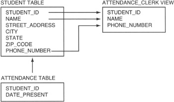
Figure 7.2: Attendance clerk database view derived from a single table

Although the student database has seven fields, the attendance clerk sees only three on his screen: STUDENT_ID, NAME, and PHONE_NUMBER. Since the attendance clerk is to call the homes of only the students absent from school, you would write a query that selected the rows of the STUDENT table that did not have a matching row in the ATTENDANCE table. Then you would have your query display only the three fields shown in the ATTENDANCE_CLERK view in Figure 7.2. Thus, the attendance clerk would see only the STUDENT_ID, NAME, and PHONE_NUMBER fields of absent students.

Now, suppose you needed to print the class schedule for the students. Well, each student needs only his or her own class information, as show in Figure 7.3.

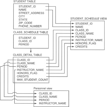
Figure 7.3: Student schedule and personnel views derived from multiple tables

The STUDENT_SCHEDULE view includes the majority of columns from the CLASS_ DETAIL table and only two columns from the STUDENT_TABLE. Thus, one student's view of the database is very different than that shown to the attendance clerk. While the attendance clerk sees the database as a list of names and phone numbers of students absent on a particular day, the student sees the database as a list of classes he is scheduled to attend. As such, you can hide table columns from view, combine columns from multiple tables, and display only some of the rows in one or more tables.

As far as the user is concerned, the view itself is a table. As mentioned previously in the current example, the student thinks there is a table with his name and class schedule, and the attendance clerk thinks there is a table of absent students. In addition to displaying data as if it were a table, a view also allows a user with update access to change values in the base tables. (Base tables are those tables from which the view [or virtual table] is derived.) Notice the PERSONNEL view shown in Figure 7.3. Suppose that you had a personnel clerk responsible for entering the names of the instructors for each of the classes. The clerk's screen (view) would show the information on a particular class and allow the clerk to update the name of the instructor for that class. When the clerk changes the name in the INSTRUCTOR_NAME column of the PERSONNEL view, the DBMS actually updates the value in the INSTRUCTOR_NAME column of the CLASS_DETAIL table in the row from which the PERSONNEL view was derived.

Schemas

The database schema is a set of tables (often called the system catalog) that contain a full description of the entire database. Although Figure 7.1 shows the names of the columns as part of the table, and Figure 7.2 and Figure 7.3 show the names of the columns in place of data, actual database data tables contain only data values. Thus, the actual database table shown in Figure 7.1 would have only the information shown below the column headings. Similarly, the table rows (or records) represented by the rectangles in Figure 7.2 and Figure 7.3 would have the actual student, attendance, and class information. The database schema has tables that contain:

• The name of each data table
• The names of each data table's columns, the type of data the column can hold, and the range of values that a column can take on
• A list of database views, how the views are derived, and which users are allowed to use which views
• A list of constraints, or rules, that limit the range of values one can enter into a column, rows one can delete from a table, and rows one can add
• Security information on who can view (query) an existing table, remove a table, or create a new one
• Security information on who can update each table's contents and which columns he or she can change
• Security information on who can add rows to or delete rows from each table

You will learn more about the database schema in Tip 12, "Understanding Schemas." For now, the important thing to know is that the database schema contains a complete description of the database.

Domains

Each column of a table (or attribute of a relation) contains some finite number of values. The domain of the table column (or attribute) is the set of all possible values one could find in that column. Suppose, for example, that you had a table of coins in a U.S. coin collection. The DENOMINATION column could have only the values 0.01, 0.05, 0.10, 0.25, 0.50, and 1.00. Thus, the "domain" of the DENOMINATION table is [0.01, 0.05, 0.10, 0.25, 0.50, 1.00], and all of the rows in the table must have one of these values in the DENOMINATION column.

Constraints

Constraints are the rules that limit what can be done to the rows and columns in a table and the values that can be entered into a table's attributes (columns). While the domain is the range of all values that a column can assume, a column constraint (such as the CHECK constraint, which you will learn about in Tip 193, "Using the CHECK Constraint to Validate a Column's Value") is what prevents a user from entering a value outside the column's domain.

In addition to limiting the values entered into a field, constraints specify rules that govern what rows can be added to or removed from a table. For example, you can prevent a user from adding duplicate rows to a table by applying the PRIMARY KEY constraint (which you will learn about in Tip 173, "Understanding Foreign Keys") to one of a table's columns. If you apply the PRIMARY KEY constraint to the STUDENT_ID column of the STUDENT table in Figure 7.1, the DBMS will make sure that every value in the STUDENT_ID column remains unique. If you already have a STUDENT_ID 101 in the STUDENT table, no user (or application program) can add another row with 101 in the STUDENT_ID column to the table. Similarly, you can apply the FOREIGN KEY constraint (which you will learn about in Tip 174, "Understanding Referential Data Integrity Checks and Foreign Keys") to a column to prevent related rows in another table from being deleted. Suppose, for example, that you had a CUSTOMER and ORDER table similar to that shown in Figure 7.4.

CUSTOMER table
CUSTOMER_ID	NAME	ADDRESS
10	Konrad King	765 Wally Way

ORDER table
Order_No	CUSTOMER_ID	Item	Quantity	Order Date
1	10	789	12	4/12/2000
2
3
4
5

Figure 7.4: ORDER and CUSTOMER table related by CUSTOMER_ID

The rows (or records) in the ORDER table are related to the CUSTOMER table by the value in the CUSTOMER_ID column. Thus, a row (or order) in the ORDER table with a CUSTOMER_ID of 10 was placed by Customer 10 (the row in the CUSTOMER table with a 10 in the CUSTOMER_ID column). If someone removed Customer 10 from the CUSTOMER table, you would no longer have any information (other than customer number) on the person that placed Order 1. You can prevent the loss of information by placing the FOREIGN KEY constraint on the CUSTOMER_ID column of the ORDER table. Once in place, the constraint will prevent anyone from deleting Customer 10 from the CUSTOMER table, as long as at least one row (order) in the ORDER table has a 10 in the CUSTOMER_ID field.

In short, constraints are the rules that maintain the domain, entity, and referential integrity of your database. You will learn all about the database integrity and the importance of maintaining it in Tips 175–190.

Understanding the Components of a Table

An SQL table consists of scalar (single-value) data arranged in columns and rows. Relational database tables have the following components:

• A unique table name
• Unique names for each of the columns in the table
• At least one column
• Data types, domains, and constraints that specify the type of data and its range of values for each column in the table
• A structure in which data in one column of the table has the same meaning in every row of the table
• Zero or more rows that represent physical or logical entities

When naming a table, bear in mind that no two tables you create can have the same name. However, table names in the SQL database need be unique only among all of the tables created (or owned) by an individual user. As such, if two users—Joe and Mark, for example—were to create tables in an SQL database, both of them could create a table named Stocks. However, neither of them could create two tables named Stock in the same schema. In Tip 9, "Understanding Table Names," you'll learn more about table names and how the DBMS uses the owner name and schema name to make the names unique across all of the tables in the database. For now, the important thing to know is that you must give your table a name, and you don't have to worry about what other people have named their tables. When selecting a table name, analyze the columns you plan to include in the table, and use a name that summarizes the table's contents. Figure 8.1, for example, contains columns of data that deal with phone call data: PHONE_REP_ID (who made the call), PHONE_NUMBER (the phone number called), DATE_TO_CALL and TIME_TO_CALL (the date and time the call was to be made), DATE_CALLED and TIME_CALLED (the date and time the call was made), HANGUP_TIME (the time the call ended), and DISPOSITION (what happened as a result of the call). The column titles indicate that the table will contain phone call data. Therefore, CALL_HISTORY is an appropriate table name since the name describes the type of data that can be retrieved from the table.

CALL_HISTORY table
PHONE_REP_ID	PHONE_NUMBER	DATE_TO_CALL	TIME_TO_CALL	DATE_CALLED	TIME_CALLED	HANGUP_TIME	DISPOSITION

Figure 8.1: Relational database table of phone call history data

Each horizontal row in a relational database table represents a physical or logical entity. In the CALL_HISTORY table, for example, each row represents a phone call. The columns in a row represent data items. Although neither the relational database rules nor the SQL-92 specification dictates that columns in a table must be somehow related, you will seldom (if ever) see a database table where the columns are just a random mix of data. Typically (if not by convention), data in the columns of a row details the attributes of the entity represented by that row. Notice that the columns in the CALL_HISTORY table shown in Figure 8 all describe some attribute of a phone call.

All relational database tables have at least one column. (A table may have no rows but must have at least one column.) The SQL standard does not specify the maximum number of columns, but most commercial databases normally limit the number of columns in a table to 255. Similarly, the SQL standard places no limit on the number of rows a table may contain. As a result, most SQL products will allow a table to grow until it exhausts the available disk space—or, if they impose a limit, they will set it to a number in the billions.

The order of the columns in a table has no effect on the results of SQL queries on the database. When creating a table, you do, however, have to specify the order of the columns, give each column a unique name, specify the type of data that the column will contain, and specify any constraints (or limits) on the column's values. To create the table shown in Figure 8.1, you could use this SQL statement:

 CREATE TABLE CALL_HISTORY
 (PHONE_REP_ID CHAR(3) NOT NULL,
 PHONE_NUMBER INTEGER NOT NULL,
 DATE_TO_CALL DATE,
 TIME_TO_CALL INTEGER,
 DATE_CALLED DATE NOT NULL,
 TIME_CALLED INTEGER NOT NULL,
 HANGUP_TIME INTEGER NOT NULL,
 DISPOSITION CHAR(4) NOT NULL)

When you look vertically down the columns in a relational database table, you will notice that the column data is self-consistent, meaning that data in the column has the same meaning in every row of the column. Thus, while the order of the columns is immaterial to the query, the table must have some set arrangement of columns that does not change from row to row. After you create the table, you can use the ALTER TABLE command to rearrange its columns; doing so will have no effect on subsequent SQL queries on the data in the table.

Each column in the table has a unique name, which you assign to the column when you execute the CREATE TABLE statement. In the current example, the column heading names are shown at the top of each column in Figure 8.1. Notice that the DBMS assigns column names from left to right in the table and in the order in which the names appear in the CREATE TABLE statement. All of the columns in a table must have a different (unique) name. However, the same column name may appear in more than one table. Thus, I can have only one PHONE_NUMBER column in the CALL_HISTORY table, but I can have a PHONE_NUMBER column in another table, such as CALLS_TO_MAKE, for example.

Understanding Table Names

When selecting the name for a table, make it something short but descriptive of the data the table will contain. You will want to keep the name short since you will be typing it in SQL statements that work with the table's data. Keeping the name descriptive will make it easy to remember which table has what data, especially in a database system with many (perhaps hundreds) of tables. If you are working on a personal or departmental database, you normally have carte blanche to name your tables whatever you wish—within the limits imposed by your DBMS, of course. SQL does not specify that table names begin with a certain letter or set of letters. The only demand is that table names be unique by owner. (We'll discuss table ownership further in a moment.) If you are working in a large, corporatewide, shared database, your company will probably have some restrictions on table names to organize the tables by department (perhaps) and to avoid name conflicts. In a large organization, for example, tables for sales may all begin with "SALES_," those for human resources might begin with "HR_," and those for customer service might start with "SERVICE_." Again, SQL makes no restrictions on the table names other than they be unique by owner—a large company with several departments may want to define its own set of restrictions to make it easier to figure out where the data in a table came from and who is responsible for maintaining it.

In order to create a table, you must be logged in to the SQL DBMS, and your username must have authorization to use the CREATE TABLE statement. Once you are logged in to the DBMS, the system knows your username and automatically makes you the owner of any table you create. Therefore, if you are working in a multi-user environment, the DBMS may indeed have more than one table named CUSTOMER—but it has only one CUSTOMER table owned by any one user. Suppose, for example, that DBMS users Karen and Konrad each create a CUSTOMER table. The DBMS will automatically adds the owner's name (by default, the table owner is the user ID of the person creating the table) to the name of the table to form a qualified table name that is then stored in the system catalog. Thus, Karen's CUSTOMER table would be stored in the system catalog as KAREN.CUSTOMER, and Konrad's table would be stored as KONRAD.CUSTOMER. As such, all of the table names in the system catalog are still unique even though both Konrad and Karen executed the same SQL statement: CREATE TABLE CUSTOMER.

When you log in to the DBMS and enter an SQL statement that references a table name, the DBMS will assume that you are referring to a table that you created. As such, if Konrad logs in and enters the SQL statement SELECT * FROM CUSTOMER, the DBMS will return the values in all columns of all rows in the KONRAD.CUSTOMER table. Likewise, if Karen logs in and executes the same statement, the DBMS will display the data in KAREN.CUSTOMER. If another user (Mark, for example) logs in and enters the SQL statement SELECT * FROM CUSTOMER without having first created a CUSTOMER table, the system will return an error, since the DBMS does not have a table named MARK.CUSTOMER.

In order to work with a table created by another user, you must have the proper authorization (access rights), and you must enter the qualified table name. A qualified table name specifies the name of the table's owner, followed by a period (.) and then the name of the table (as in .

). In the previous example, if Mark had the proper authorization, he could type the SQL statement SELECT * FROM KONRAD.CUSTOMER to display the data in Konrad's CUSTOMER table, or SELECT * FROM KAREN.CUSTOMER to display the contents of Karen's CUSTOMER table. You can use a qualified table name in an SQL statement wherever a table name can appear.

The SQL-92 standard further extends the DBMS's ability to work with duplicate tables by allowing a user to create tables within a schema. (You will learn more about schemas in Tip 12, "Understanding Schemas," and about creating tables within schemas in Tip 506, "Using the CREATE SCHEMA Statement to Create Tables and Grant Access to Those Tables.") The fully qualified name of a table created within a schema becomes the schema name, followed by a period (.) and then the name of the table (for example, .

). Thus an individual user could create multiple tables with the same name by putting each of the tables in a different schema. For now, the important thing to know is that every table must have a unique qualified table name. As such, a user cannot use the same name for two tables unless he creates the tables in different schemas (which you will learn how to do in Tip 506).

Understanding Column Names

The SQL DBMS stores the names of the columns along with the table names in its system catalog. Column names must be unique within a table but can appear in multiple tables. For example, you can have a STUDENT_ID column in both a STUDENT table and a CLASS_SCHEDULE table. However, you cannot have more than one STUDENT_ID column in either table. When selecting a column name, use a short, unique (to the table being created) name that summarizes the kind of data the column will contain. If you plan to store an address in a column, name the column ADDRESS or STREET_ADDRESS, use CITY as the name for a column that holds the city names, and so on. The SQL specification does not limit your choice as to the name you use for a column (other than that a column name can appear only once in any one table). However, using descriptive column names makes it easier to know which columns to use when you write SQL statements to extract data from the table.

When you specify a column name in an SQL statement, the DBMS can determine the table to which you are referring if the column name is unique to a single table in the statement. Suppose, for example, that you had two tables with column names defined as shown in Figure 10.1.

STUDENT table

STUDENT_ID

STUDENT_NAME

STREET_ADDRESS

CITY

STATE

ZIP_CODE

PHONE_NUMBER

CLASS1_TEACHER

CLASS2_TEACHER

CLASS3_TEACHER

CLASS4_TEACHER

TEACHER table

TEACHER_ID

TEACHER_NAME

SUBJECT

PHONE_NUMBER

Figure 10.1: Example STUDENT table and TEACHER table with duplicate column names

The DBMS would have no trouble determining which columns to display in the following SQL statement:

 SELECT
 STUDENT_ID, STUDENT_NAME, SUBJECT, TEACHER_NAME
 FROM
 STUDENT, TEACHER
 WHERE
 CLASS1_TEACHER = TEACHER_ID

Since STUDENT_ID and STUDENT_NAME appear only in the STUDENT table, the DBMS would display the values in the STUDENT_ID and STUDENT_NAME columns of the STUDENT table. Similarly, SUBJECT and TEACHER_NAME are found only in the TEACHER table, so the DBMS would display SUBJECT and TEACHER_NAME information from the TEACHER table as it executes the SELECT statement. Thus, if you use columns from more than one table in an SQL statement, the DBMS can figure out which column name refers to which table if none of the column names in the SQL statement appears in more than one table listed in the FROM clause.

If you want to display data from one or more columns that have the same name in more than one table used in an SQL statement, you will need to use the qualified column name for each of the duplicate columns. The qualified column name is the name of the table, followed by a period (.) and then the name of the column. As such, if you wanted to list the student's phone number (found in the PHONE_NUMBER column in the STUDENT table), you could use the following SQL statement:

SELECT
 STUDENT_ID, STUDENT_NAME, STUDENT.PHONE_NUMBER, SUBJECT,
 TEACHER_NAME
FROM
 STUDENT, TEACHER
WHERE
 CLASS1_TEACHER = TEACHER_ID

If you specified only PHONE_NUMBER after STUDENT_NAME, the DBMS would not know if it were supposed to display the student's phone number or the teacher's phone number, since both tables have the column named PHONE_NUMBER. By using the qualified column name (STUDENT.PHONE_NUMBER, in this example), you specify not only the column whose data you want, but also the table whose data the DBMS is to use. In general, you can use qualified column names in an SQL statement wherever unqualified column names can appear.

As you learned in Tip 9, "Understanding Table Names," you need to use qualified table names whenever you want to work with a table that you do not own. Thus, you must use the qualified table name (the name of the table, followed by a period [.] and then the table name) in your SQL statement wherever the name of the table that you do not own appears. Thus, in the current example, if you own the TEACHER table but you did not create the STUDENT table (and Konrad, who created the table, gave you access to the table but did not assign its ownership to you), you would modify the SQL statement as follows:

SELECT
 STUDENT_ID, STUDENT_NAME, KONRAD.STUDENT.PHONE_NUMBER,
 SUBJECT, TEACHER_NAME
FROM
 KONRAD.STUDENT, TEACHER
WHERE
 CLASS1_TEACHER = TEACHER_ID

By using the qualified table name KONRAD.STUDENT in place of STUDENT in the SELECT statement, you tell the DBMS to extract data from the STUDENT table owned by Konrad instead of trying to get data from a nonexistent STUDENT table created (or owned) by you.

Understanding Views

As you learned in Tip 7, "Understanding Terms Used to Define an SQL Database," views are virtual tables. A view looks like a table because it appears to have all of the essential components of a table-it has a name, it has rows of data arranged in named columns, and its definition is stored in the database catalog right along with all of the other "real" tables. Moreover, you can use the name of a view in many SQL statements wherever a table name can appear. What makes a view a virtual vs. real table is that the data seen in a view exists in the tables used to create the view, not in the view itself.

The easiest way to understand views is to see how they are created, what happens when you use the name of a view in an SQL query, and what happens to the view upon completion of the SQL statement.

To create a view, use the SQL CREATE VIEW statement. Suppose, for example, that you have relational database tables with salesman and payroll data similar to that shown in Figure 11.1.

SALES_REPS table
EMP_NUM	NAME	APPT_COUNT	SALES_COUNT	SSAN	ADDR
1	Tamika James	10	6
2	Sally Wells	23	9
3	Robert Hardy	17	12
4	Jane Smith	12	8
5	Rodger Dodger	22	17
6	Clide Williams	19	16

PAYROLL table
EMP_NUM	YTD_SALARY	YTD_COMMISSION
1	$69,595.00	$2,595.00
2	$89,498.00	$16,323.00
3	$45,000.00	$27,123.00
4	$75,000.00	$17,000.00
5	$63,000.00	$5,000.00
6	$72,898.00	$2,993.00

Figure 11.1: Example relational database tables to use as base tables for a view

When you execute this SQL statement

CREATE VIEW APPT_SALES_PAY
 (NAME,APPTS,SALES,SALES_PCT,YTD_SALARY,YTD_COMMISSION) AS
SELECT
 NAME, APPT_COUNT, SALES_COUNT, ((APPT_COUNT / SALES_COUNT)
 * 100), YTD_SALARY, YTD_COMMISSION
FROM
 SALES_REPS, PAYROLL
WHERE
 SALES_REPS.EMP_NUM = PAYROLL.EMP_NUM

the DBMS stores the definition of the view in the database under the name APPT_SALES_PAY. Unlike the CREATE TABLE statement that creates an actual empty database table in addition to storing the definition of the table in the system catalog, the CREATE VIEW statement only stores the definition of the view.

The DBMS does not create an actual table when you create a view because, unlike a real table, the view does not exist in the database as a set of values in a table. Instead, the rows and columns of data you see through a view are the results produced by the query that defines the view.

After you create a view, you can use it in a SELECT statement as if it were a real table. For example, after you create the APPT_SALES_PAY view (using the CREATE statement that follows Figure 11.1), you can display the results of the query that defines the view by using this SQL statement:

 SELECT * FROM APPT_SALES_PAY

When the DBMS sees the reference to a view in an SQL statement, it finds the definition of the view in its system tables. The DBMS then transforms the view references into an equivalent request against the base tables and executes the equivalent SQL statements. For the current example, the DBMS will execute a multi-table select statement (which you will learn about in Tip 205, "Using a SELECT Statement with a FROM Clause for Multi-table Selections") to form the virtual table shown in Figure 11.2, and then display the values in all of the columns in each row of the virtual table.

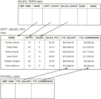
Figure 11.2: APPT_SALES_PAY view generated from base tables SALES_REPS and PAYROLL

For simple views, the DBMS will construct each row of the view's virtual table "on the fly." Thus, in the current example, the DBMS will extract data from the columns specified in the view definition from one row in the SALES_REPS and PAYROLL tables to create a row in the virtual APPT_SALES_PAY table. Next, the DBMS will execute the SELECT statement to display the fields in the newly created row (of the virtual table). The DBMS will then repeat the procedure (create a virtual row from the two tables and then display the columns of the virtual row), until no more rows in the base tables satisfy the query in the view.

To execute more complex views (such as those used in SQL statements that update data in the base tables), the DBMS must actually materialize the view, meaning that the DBMS will perform the query that defines the view and store the results in a temporary table. The DBMS will then use the temporary table to execute the SQL statement (such as SELECT * FROM APPT_SALES_PAY) that references the view. When the DBMS no longer needs the temporary table (at the completion of the SQL statement), the DBMS discards it. Remember, views do not hold data; they merely display the data stored in their base tables (SALES_REPS and PAYROLL, in the current example).

Whether the DBMS handles a particular view by creating rows on the fly or by pulling the view data into a temporary table, the end result is the same-the user can reference views in SQL statements as if they were real tables in the database.

There are several advantages in using views:

• Provide security. When you don't want a user to see all of the data in a table, you can use a view to let the user see only specific columns. Thus, someone working in the personnel department can see the employee name and address information through a view, while the salary or hourly pay can remain hidden by being excluded from the view.
• Simplify data structures. You can present the database as a "personalized" set of tables. Suppose, for example, that you have separate employee and payroll tables. You can use a view to display employee names and pay figures in a single virtual table for the company's managers.
• Abstract data structures. As time goes on, some users will save SQL queries that they use often, and others may even write Visual Basic or C++ programs that extract data from the database to produce reports. If someone (such as the table owner or database administrator) changes the physical structure of a table by splitting it into two tables, for example, saved user queries may no longer function and application programs may try to access columns that no longer exist. However, if users write their queries or application programs to access data in the "virtual" view tables, you can insulate them from changes to the underlying database structures. When you split a table, for example, you need change the view's query so that it recombines the split tables into the set of columns found in the original view.
• Simplify queries. By using a view to combine the data from several tables into a single virtual table, you make it possible for a user to write SQL queries based on a single table, thus avoiding the complexity of using multi-table SELECT and JOIN statements.

While views provide several advantages, there are two main disadvantages to using them:

• Performance. Since a view is a virtual table, the DBMS must either materialize the data in a view as a temporary table or extract the data in the view's rows on the fly (one row at a time) whenever you use a view in an SQL statement. Thus, each time you use an SQL statement that contains a view reference, you are telling the DBMS to perform the query that defines the view in addition to performing the query or update in SQL statement you just entered.
• Update restrictions. Unfortunately, SQL violates Rule 6 of Codd's rules (you learned about this in Tip 6, "Understanding Codd's 12-Rule Relational Database Definition"), in that not all views are updateable. Currently, SQL limits updateable views to those based on queries on a single table without GROUP BY or HAVING clauses. In addition, to be updateable a view cannot have aggregate functions, calculated columns, or a SELECT DISTINCT clause. And, finally, the view must contain a table key column, and any columns excluded from the view must be NULL-able in the base table.

Due to SQL limitations on what views you can use for updating base tables, you cannot always create views to use in place of base tables. Moreover, in those cases where you can use a view, always weigh the advantages of using the view against the performance hit you take in having the DBMS create virtual tables every time it executes an SQL statement that references a view.

Understanding Schemas

A table consists of rows and columns of data that deal with a specific type of entity such as marketing calls, sales statistics, customers, orders, payroll, and so on. A schema is the collection of related tables. Thus, a schema is to tables what tables are to individual data items. While a table brings together related data items so that they describe an entity when considered a row at a time in a table, the schema is the set of related tables and organizational structure that describe your department or company.

Suppose that you worked in a sales organization with five departments as shown in Figure 12.1.

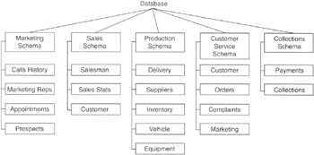
Figure 12.1: Database with tables grouped into five schemas, one for each department in the company

The tables in the marketing department, for example, might include tables showing the history of marketing calls made, marketing representative appointment setting statistics, an appointment list, and demographic data on prospects. The collections department, meanwhile, would have tables that deal with customer information, payments made on accounts, and collections activity such as scheduling dunning letters and field calls for payment pickups. All of the tables shown in Figure 12.1 would exist in a single database. However, each department has its own set of activities, as reflected in the set tables of data it maintains. Each department's tables could be organized into a separate schema within the company's database.

The schema is more of a "container" for objects than just a "grouping" of related tables because a schema includes:

• Tables. Related data items arranged in columns of rows that describe a physical or logical entity. The schema includes the tables as well as all of the components of a table (described in Tip 8, "Understanding the Components of a Table"), which include the column domains, check constraints, primary and foreign keys, and so on).
• Views. Virtual tables defined by an SQL query that display data from one or more base tables (as described in Tip 11, "Understanding Views"). The schema includes the definition of all views that use base tables of "real" data included in the schema. (As you learned in Tip 11, the virtual tables exist only for the duration of the SQL statement that references the view.)
• Assertions. Database integrity constraints that place restrictions on data relationships between tables in a schema. You will learn more about assertions in Tip 33, "Understanding Assertions."
• Privileges. Access rights that individual users and groups of users have to create or modify table structures, and to query and/or update database table data (or data in only specific columns in tables through views). You will learn all about the SQL security privileges in Tips 135-158.
• Character sets. Database structures used to allow SQL to display non-Roman characters such as Cyrillic (Russian), Kanji (Asian), and so on.
• Collations. Define the sorting sequences for a character set.
• Translations. Control how text character sequences are to be translated from one character set to another. Translations let you store data in Kanji, for example, and display it in Cyrillic, Kanji, and Roman-depending on the user's view of the data. In addition to showing which character(s) in one character set maps to which character(s) in another, translations define how text strings in one character set compare to text strings in another when used in comparison operations.

In short, the schema is a container that holds a set of tables, the metadata that describes the data (columns) in those tables, the domains and constraints that limit what data can be put into a table's columns, the keys (primary and foreign) that limit the rows that can be added to and removed from a table, and the security that defines who is allowed to do what to objects in the schema.

When you use the CREATE TABLE statement (which you will learn about in Tip 46, "Using the CREATE TABLE Statement to Create Tables"), the DBMS automatically creates your table in the default schema for your interactive session, the schema named . Thus, if users Konrad and Karen each log in to the database and execute the SQL statement

CREATE TABLE CALL_HISTORY
 (PHONE_REP_ID CHAR(3) NOT NULL,
 PHONE_NUMBER INTEGER NOT NULL,
 DATE_TO_CALL DATE,
 TIME_TO_CALL INTEGER,
 DATE_CALLED DATE NOT NULL,
 TIME_CALLED INTEGER NOT NULL,
 HANGUP_TIME INTEGER NOT NULL,
 DISPOSITION CHAR(4) NOT NULL)

the DBMS will add a table to each of two schemas, as shown in Figure 12.2.

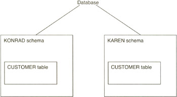
Figure 12.2: Database with two schemas, KONRAD and KAREN

In short, anytime you use the CREATE statement to create a database object such as a table, view, domain, assertion, and so on, the DBMS will create that object in the default "container" schema.

If you want to create an object in a specific schema "container," the container must exist and you must use the qualified name for the object you are creating. Qualified object names are an extension of the qualified table names you learned about in Tip 9, "Understanding Table Names." Instead of using ., use .to place an object in a specific schema.

For example, to create the MARKETING schema shown in Figure 12.1, you could use the SQL statement

 CREATE SCHEMA MARKETING AUTHORIZATION KONRAD
 CREATE TABLE CALLS_HISTORY
 (PHONE_REP_ID CHAR (3) NOT NULL,
 PHONE_NUMBER INTEGER, NOT NULL,
 DATE_CALLED DATE)
 CREATE TABLE MARKETING REPS
 (REP_ID CHAR(3),
 REP_NAME CHAR(25))
 CREATE TABLE APPOINTMENTS
 (APPOINTMENT_DATE DATE,
 APPOINTMENT_TIME INTEGER,
 PHONE_NUMBER INTEGER)
 CREATE TABLE PROSPECTS
 PHONE_NUMBER INTEGER,
 NAME CHAR(25),
 ADDRESS CHAR(35))

to create the MARKETING schema and the structure for its four tables. The AUTHORIZATION predicate in the CREATE SCHEMA statement authorizes Konrad to modify the schema and its objects. As such, Konrad could then use an ALTER TABLE MARKETING.

statement to change the columns, domains, and constraints of columns in the tables included in the MARKETING schema. Moreover, Konrad can create additional tables in the MARKETING schema by specifying the schema name in a CREATE TABLE statement, such as:

 CREATE TABLE MARKETING.CONTESTS
 (DESCRIPTION CHAR(25),
 RULES VARCHAR(100),
 WIN_LEVEL1 MONEY,
 WIN_LEVEL2 MONEY,
 WIN_LEVEL3 MONEY)

All DBMS products have schema, or "containers," that hold a collection of tables and related objects. However, the name you can give to a schema varies from product to product. Oracle, Informix, and Sybase, for example, require that the schema name and username be the same. Each also limits the types of objects you can define in the CREATE SCHEMA statement. Thus, you must check the syntax of the CREATE SCHEMA statement in your DBMS manual (or Help system) to see what objects can be grouped together in schema "containers" and what names you can give to schema itself.

Understanding the SQL System Catalog

The system catalog is a collection of tables that the DBMS itself owns, creates, and maintains in order to manage the user-defined objects (tables, domains, constraints, schemas, other catalogs, security, and so on) in the database. As a collection, the tables in the system catalog are often referred to as the system tables because they contain data that describes the structure of the database and all of its objects and are used by the database management system in some way during the execution of every SQL statement.

When processing SQL statements, the DBMS constantly refers to the tables in the system catalog to:

• Make sure that all tables or views referenced in a statement actually exist in the database
• Make sure the columns referenced in the SQL statement exist in the tables listed in the target tables list portion of the statement (for example, the FROM section of a SELECT statement)
• Resolve unqualified column names to one of the tables or views referenced in the statement
• Determine the data type of each column
• Check the system security tables to make sure that the user has the privilege necessary to carry out the action described in the SQL statement on the target table (or column)
• Find and apply any primary key, foreign key, domain, and constraint definitions during INSERT, UPDATE, or DELETE operations

By storing the database description as a set of system tables, SQL meets the requirement for a "Dynamic Online Catalog Based on the Relational Model," listed as Rule 4 of Codd's 12 rules that define a relational database (which you learned about in Tip 6, "Understanding Codd's 12-Rule Relational Database Definition").

Not only does an SQL database use the system tables in the system catalog to validate and then execute SQL statements issued by the user or application programs, but the DBMS also makes the data in the system catalog available either directly or through views.

Note 

The database administrator may limit access to the tables in the system catalog due to security concerns. After all, if you knew the primary key constraints, column name, and data domains for a particular table, you could determine the contents of the column(s) in the primary key-even if you did not have SELECT access to the table itself. Moreover, the structure of the database may itself be a trade secret if table and/or column names give information as the types of data a company in a particular market would find important enough to collect.

Since the DBMS maintains the data in the system tables so that it accurately describes the structure and contents of the database, user access to the system catalog is strictly read-only. Allowing a user to change the values in system tables would destroy the integrity of the system catalog. After all, if the DBMS is doing its job of maintaining the tables to accurately describe the database, any changes made to the catalog by the user would, by definition, change a correct value into an incorrect one.

The main advantage of user-accessible system tables is that they allow applications programmers to write general-purpose database tools that allow users to access SQL databases without having to know SQL. For example, by querying the system tables, an application program can determine the list of tables and views to which a user has access. The program could then allow the user to select the table(s) of interest and list the columns available for display in the selected table(s). Next the application program could allow the user to enter any "filtering" or search criteria. After the user has selected the table and columns and entered selection criteria, the application program could generate the SQL statements necessary to extract the data and format and display the query results to the user.

Without the system tables, the table and column names and the access rights would have to be hard-coded into the application programs, making general-purpose third-party applications impossible to write. Due to the demand for such third-party software solutions (owing perhaps to the scarcity of good SQL programmers), most major SQL database products are moving to support a common a set of system catalog views know collectively as the INFORMATION_SCHEMA.

You will learn more about the INFORMATION_SCHEMA and system tables in Tips 472-493, which discuss the INFORMATION_SCHEMA and the system tables on which it is based, and Tip 494 "Understanding the MS-SQL Server System Database Tables," which reviews the MS-SQL Server system tables. For now, the important thing to know is that the INFORMATION_SCHEMA views will allow the same application program to access system table information in different database products even though the structure of the catalog and the tables it contains varies considerable from one brand of DBMS to another.

Understanding Domains

A domain is the set of all values that are legal for a particular column in a table. Suppose, for example, that your EMPLOYEE table had a DEPENDANT field that your company policy states must be an INTEGER between 0 and 14. The domain of DEPENDANT would then be 0,1,2,3,4,5,6,7,8,9,10,12,13,14. Or, suppose you were maintaining a table for a tablecloth inventory that has a COLOR column, and all of your tablecloths were white, beige, or blue. The domain of the COLOR column would then be WHITE, BEIGE, BLUE.

Once you define a domain using the CREATE DOMAIN statement (which we will discuss in Tip 170, "Using the CREATE DOMAIN Statement to Create Domains"), you can use the domain as a data type when defining a column. Suppose, for example, that you had a CUSTOMER table with a STATE field. You could define the domain of the STATE field by creating a STATE_CODE domain using this SQL statement:

 CREATE DOMAIN STATE_CODE AS CHAR(2)
 CONSTRAINT VALID_STATE_ABBREVIATION
 CHECK (VALUE IN ('AL', 'AK', 'AZ', 'CO', 'CT', ... ))

Note 

You would list the remaining 45 state codes in place of the "..." in the VALUE IN section of the CREATE DOMAIN statement.

To have the DBMS validate data as it is entered into the STATE field of the CUSTOMER table, use the STATE_CODE domain as the data type for the state field when creating the table, as shown in this SQL statement:

 CREATE TABLE CUSTOMER
 (NAME VARCHAR(25),
 ADDRESS VARCHAR(35),
 CITY VARCHAR(20),
 STATE STATE_CODE,
 ZIP CODE INTEGER)

The beauty of defining a domain is that you can change it on the fly without having to alter the structure of the table or recompile any existing stored procedures or application programs.

Suppose, for example, that Puerto Rico were to become a state; you could use the ALTER DOMAIN statement to add PR to the list of valid state abbreviations. The DBMS would then automatically allow the user to enter PR for the STATE field, since the updated STATE_CODE domain (stored in the system tables) would include PR as a valid state code the next time the DBMS referred to it in checking the value in the STATE field of a row to be added to the CUSTOMER table.

Understanding Constraints

Constraints are database objects that restrict the data that a user or application program can enter into the columns of a table. There are seven types of constraints: assertions, domains, check constraints, foreign key constraints, primary key constraints, required data, and uniqueness constraints. Each type of constraint plays a different roll in maintaining database integrity:

• Assertions. Allow you to maintain the integrity of a relationship among data values that cross multiple tables within a database. Suppose, for example, that you have a marketing room with four teams of sales representatives, and each of the sales representatives has a quota for the number of sales he or she is to make on a daily basis. If your marketing manager has a daily quota, you would use an assertion to ensure that the ROOM_QUOTA column in the marketing manager record (row) of the MANAGER table did not exceed the sum of the values in the REP_QUOTA column in the PHONE_REP table. You will learn more about assertions in Tip 33, "Understanding Assertions," and Tip 199, "Using the CREATE ASSERTION Statement to Create Multi-table Constraints."
• Domains. Ensure that users and applications enter only valid values into table columns. Every column in a table has a certain set of values that are legal for that column. For example, if the MONTHLY_SALARY column in a PAYROLL table must always have values between $0.00 and $100,000.00, you can apply a domain constraint to tell the DBMS to prevent values outside of that range from being entered into the database. (Of course, high-stress jobs, such as SQL DBA, will require that the upper limit of the MONTHLY_SALARY domain be higher.)
• Check constraints. In addition to being used to define domains and assertions, this constraint can be applied directly to table columns in CREATE TABLE or ALTER TABLE statements. Whether a check constraint is given a name (using the CREATE DOMAIN or CREATE ASSERTION statement) or is added directly to a table definition, it performs the same function.

As you learned in Tip 14, "Understanding Domains," you create a domain by giving a name to a check constraint with a constant set of data values. Instead of using the CREATE DOMAIN statement, you can include CHECK constraint (which you will learn about in Tip 193, "Using the CHECK Constraint to Validate a Column's Value") directly to a column in the CREATE TABLE or ALTER TABLE statement.

As you will learn in Tip 33, an assertion is really another name for a CHECK constraint to which you've assigned a name using the CREATE ASSERTION statement. You can use assertions or multi-table CHECK constraints to apply business rules to the values of columns in a table. Suppose, for example, that your company did not allow back orders. As such, you could use a query in the CHECK constraint on the QUANTITY column of the ORDER table that would allow only values that were less than the total of the product currently on hand, as shown in the INVENTORY table. You will learn more about using search conditions in the CHECK constraint in Tip 444, "Understanding When to Use a CHECK Constraint Instead of a Trigger."

• Foreign key constraints. Are used to maintain referential integrity within the database by making sure that the parent record is not removed if there are still child records. Conversely, the FOREIGN KEY constraint also makes sure that you do not add a child record (row) to a table if there is no corresponding parent. Suppose, for example, that you had two tables, STUDENT and GRADES. You would apply the FOREIGN KEY constraint (which you will learn about in Tip 174, "Understanding Referential Data Integrity Checks and Foreign Keys") to one of the columns (such as STUDENT_NUMBER) in the child (GRADES) table to tell the DBMS that the value inserted in that column must also be present in the PRIMARY KEY column in one of the rows in the parent (STUDENT) table. Thus, if STUDENT_ID were the PRIMARY KEY in the (parent) STUDENT table, the DBMS would allow the insertion of a row into the GRADES table only if the student record (row) had a STUDENT_NUMBER equal to one of the STUDENT_IDs in the STUDENT table. Conversely, the DBMS would prevent the deletion of any student record (row) from the STUDENT table if one or more grades records (rows) had a STUDENT_NUMBER equal to the STUDENT_ID in the row to be deleted.
• Primary key constraints. Maintain entity integrity by specifying that at least one column in a table must have a unique value in each and every row of the table. Having a column with a different value in every row of the table prevents two rows of the table from being identical, thereby satisfying Codd's Rule #2 ("The Guaranteed Access Rule," discussed in Tip 6, "Understanding Codd's 12-Rule Relational Database Definition"). If you have a STUDENT table, for example, you would want one and only one row in the table to list the attributes (columns) for any one student. As such, you would apply the PRIMARY KEY constraint (which you will learn about in Tip 173, "Understanding Foreign Keys") to the STUDENT_ID column of the STUDENT table in order to ensure that no two students were given the same student ID number.
• Required data. Some columns in a table must contain data in order for the row to successfully describe a physical or logical entity. For example, suppose you had a GRADES table that contained a STUDENT_ID column. Each and every row in the table must have a value in the STUDENT_ID column in order for that grade record (row) to make sense—after all, a grade in a class is meaningless unless it is associated with the specific student (identified by the STUDENT_ID) that earned it. You will learn about the NOT NULL (required data) constraint in Tip 191, "Using the NOT NULL Column Constraint to Prevent NULL Values in a Column."
• Uniqueness constraints. While each table can have only one PRIMARY KEY, there are times when you may want to specify that more than one column in a table should have a unique value in each row. You can apply the UNIQUE constraint (which you will learn about in Tip 192, "Using the UNIQUE Column Constraint to Prevent Duplicate Values in a Column") to a table column to ensure that only one row in the table will have a certain value in that column. Suppose, for example, that you have a TEACHERS table and want to have only one teacher available for each subject offered at the school. If the table's PRIMARY KEY constraint were already applied to the TEACHER_ID column, you could apply the UNIQUE constraint to the SUBJECT column to tell the DBMS not to allow the insertion of a row where the value in the SUBJECT column matched the value in the SUBJECT column of a row already in the table.

The DBMS stores a description of each constraint in its system tables when the constraint is normally specified as part of a table definition (CHECK, FOREIGN KEY, PRIMARY KEY, NOT NULL [required data], UNIQUE), or by using the CREATE statement (ASSERTION, DOMAIN). All constraints are database objects that either limit the values that you can put into a table's columns or limit the rows (combination of column values) that you can add to a table.

Understanding the History of SQL

Both SQL and relational database theory originated in IBM's research laboratories. In June 1970, Dr. Edgar F. Codd, an IBM engineer, wrote a paper outlining the mathematical theory of how data could be stored in tables and manipulated using a data sublanguage. The article, entitled "A Relational Model of Data for Large Shared Data Banks," was published in the Communications of the Association for Computing Machinery (ACM) and led to the creation of relational database management systems (DBMS) and Structured Query Language (SQL).

After Dr. Codd published his article, IBM researchers began work on System /R, a prototype relational DBMS. During the development of System /R, the engineers also worked on a database query language-after all, once data was stored in a DBMS, it would be of no use unless you could combine and extract it in the form of useful information. One of the query languages, SEQUEL (short for Structured English Query Language), became the de facto standard data query language for relational DBMS products. The SQL we use today is the direct descendant of IBM's original SEQUEL data sublanguage.

Although IBM started the research in 1970 and developed the first prototype relational DBMS (System /R) in 1978, it was Oracle (then known as Relational Software, Inc.) that introduced the first commercial relational DBMS product in 1980. The Oracle DBMS (which ran on Digital Equipment Corp [DEC] VAX minicomputers) beat IBM's first commercial DBMS product (SQL/DS) to market by two years. While Oracle continued to refine its product and released version 3, which ran on mainframes, minicomputers, and PCs, in 1982, IBM was working on Database 2 (DB2) which it announced in 1983 and began shipping in 1985.

DB2 operated on IBM's MVS operating system on IBM mainframes that dominated the large data center market at the time. IBM called DB2 its flagship relational DBMS, and with IBM's weight behind it, DB2's SQL became the de facto standard database language.

Although initially slower than other database models (such as the hierarchical model that you learned about in Tip 3, "Understanding the Hierarchical Database Model," and the network model that you learned about in Tip 4, "Understanding the Network Database Model"), the relational model had one major advantage-you didn't need a programmer to get information from the database. The relational query languages let users pose ad hoc, English-like queries to the database and get immediate answers-without having to write a program first.

As the performance of relational DBMS products improved through software enhancements and increases in hardware processing power, they became accepted as the database technology of the future. Unfortunately, compatibility across vendor platforms was poor. Each company's DBMS included its own version of SQL. While every flavor of SQL contained the basic functionality of IBM's DB2 SQL, each extended it in ways that took advantage of the particular strengths of the vendor's relational DBMS and hardware platform.

In 1986 the American National Standards Institute (ANSI) and the International Organization for Standardization (ISO) published the first formal ANSI/ISO standard for SQL. SQL-86 (or SQL1) gave SQL "official" status as the relational DBMS data language. ANSI updated the standard in 1992 to include "popular" enhancements/extensions found across DBMS products and added a "wish list" objects and methods that a DBMS should have.

SQL-92 (or SQL2), published in ANSI Document X3.135-1992, is the most current and comprehensive definition of SQL. At present, no commercial DBMS fully supports all of the features defined by SQL-92, but all vendors are working toward becoming increasingly compliant with the standard. As a result, we are getting closer to the goal of having a data language (SQL) that is truly transportable across DBMS products and hardware platforms.

Understanding the Difference Between SQL and a Programming Language

To solve problems in a procedural programming language (such as Basic, C, COBOL, FORTRAN, and so on), you write lines of code that perform one operation after another until the program completes its tasks. The program may execute its lines of code in a linear sequence or loop to repeat some steps or branch to skip others. In any case, when writing a program in a procedural language, the programmer specifies what is to be done and how to do it.

SQL, on the other hand, is a nonprocedural language in that you tell SQL what you want to do without specifying exactly how to accomplish the task. The DBMS, not the programmer, decides the best way to perform the job. Suppose, for example, that you have a CUSTOMER table and you want a list of customers that owe you more than $1,000.00. You could tell the DBMS to generate the report with this SQL statement:

 SELECT
 NAME, ADDRESS, CITY, STATE, ZIP, PHONE_NUMBER,
 BALANCE_DUE
 FROM
 CUSTOMER
 WHERE
 BALANCE_DUE > 1000.00

If writing a procedural program, you would have to write the control loop that reads each row (record) in the table, decides whether to print the values in the columns (fields), and moves on to the next row until it reaches the end of the table. In SQL, you specify only the data you want to see. The DBMS then examines the database and decides how best to fulfill your request.

Although it is an acronym for "Structured Query Language," SQL is more than just a data retrieval tool. SQL is a:

• Data definition language (DDL), for creating (and dropping) database objects such as tables, constraints, domains, and keys.
• Data manipulation language (DML), for changing values stored in columns, inserting new rows, and deleting those you no longer want.
• Data control language (DCL), for protecting the integrity of your database by defining a sequence of one or more SQL statements as a transaction in which the DBMS must complete all statements successfully or have none of them affect the database. DCL also lets you set up the security structure for the database.
• Query language, for retrieving data.

In addition to the DDL, DML, DCL, and query functions, SQL maintains data integrity and coordinates concurrent access to the database objects. In short, SQL provides all of the tools you need for controlling and interacting with the DBMS.

Despite all that it does, SQL is not a complete computer language (like Basic, C, or FORTRAN) because it contains no block (BEGIN, END) statements, conditional (IF) statements, branch (GOTO) statements, or loop (DO, WHILE, FOR) statements. Because it lacks input statements, output statements, and common procedural language control methods, SQL is considered a data sublanguage. What SQL lacks in procedural language components, it makes up for in the database realm with statements specialized for database management and data retrieval tasks.

You can get information from an SQL database by submitting ad hoc queries during an interactive session or by embedding SQL statements in a procedural application program. Issuing queries during an interactive session is most appropriate when you want a quick answer to a specific question that you may ask only once. If, on the other hand, you need the same information repeatedly and want to control the format of the output, embedding SQL statements in an application program or having the program send SQL commands to the DBMS via a call-level interface makes the most sense.

Note 

Most major database vendors are adding procedural programming language-like features to their SQL products by allowing you to create stored procedures. Stored procedures are sequences of SQL statements that you tell the DBMS to execute by entering the stored procedure's name at the console during an interactive session, or by sending the name as a command to the DBMS within an application program. The stored procedure itself contains SQL statements and code written in the vendor's extensions to SQL that provide procedural language facilities such as BEGIN-END blocks, IF statements, functions, procedures, WHILE loops, FOR loops, and so on. Oracle, for example, extends SQL with PL/SQL and SQL *Plus, while Microsoft lets you use its Transact-SQL extensions in stored procedures.

Understanding Data Definition Language (DDL)

Data definition language (DDL) is the set of SQL statements (ALTER, CREATE, DROP, GRANT) that let you create, alter, or destroy (drop) the objects that make up a relational database. To put it another way, you use DDL to define the structure and security of a database. SQL-89 (the first ANSI/ISO standard written for SQL) defines data manipulation language (DML) and DDL as two distinct and relatively unrelated languages. Moreover, DML statements, which allow you to update the data in the database, must be available for use while users are accessing the database, for obvious reasons. SQL-89 does not require that the DBMS accept DDL statements during its normal operation. Thus, the standard allows a static database structure similar to that of the hierarchical model (see Tip 3, "Understanding the Hierarchical Database Model") and the network model (see Tip 4, "Understanding the Network Database Model").

The most basic (and powerful) DDL statement is the CREATE statement. Using CREATE, you build the database schema (which you learned about in Tip 12, "Understanding Schemas"). For example, to build a database with two schemas as shown in Figure 18.1, you could use the following SQL statements:

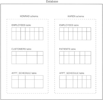
Figure 18.1: Example database with two schemas named KONRAD and KAREN, each containing three tables

CREATE SCHEMA AUTHORIZATION KONRAD
 CREATE TABLE EMPLOYEES
 (ID CHAR(3),
 NAME VARCHAR(35),
 ADDRESS VARCHAR(45),
 PHONE_NUMBER CHAR(11),
 DEPARTMENT CHAR(10),
 SALARY MONEY,
 HOURLY_RATE MONEY)
 CREATE CUSTOMERS
 (NAME VARCHAR(35),
 ADDRESS VARCHAR(45),
 PHONE_NUMBER CHAR(11),
 FOOD_PLAN CHAR(2))
 CREATE TABLE APPT_SCHEDULE
 (APPT_DATE DATE,
 APPT_TIME INTEGER,
 APPT_DISPOSITION CHAR(4),
 APPT_SALESMAN_ID CHAR(3))
GRANT SELECT, UPDATE
 ON EMPLOYEES
 TO HR_DEPARTMENT
GRANT ALL PRIVILEGES
 ON CUSTOMERS
 TO MARKETING_REPS, OFFICE_CLERKS
GRANT SELECT
 ON APPT SCHEDULE
 TO PUBLIC
GRANT SELECT, INSERT
 ON APPT SCHEDULE
 TO MARKETING REPS
CREATE SCHEMA AUTHORIZATION KAREN
 CREATE TABLE EMPLOYEES
 (ID CHARM,
 NAME VARCHAR(35),
 ADDRESS VARCHAR(45),
 PHONE_NUMBER CHAR(11),
 EMPLOYEE_TYPE CHAR (2),
 SALARY MONEY,
 HOURLY_RATE, MONEY)
 GRANT SELECT, UPDATE
 ON EMPLOYEES
 TO HR DEPARTMENT
 CREATE PATIENTS
 (ID INTEGER
 SPONSOR_SSAN CHAR(11),
 NAME VARCHAR(35),
 ADDRESS VARCHAR(45),
 PHONE_NUMBER CHAR(11),
 AILMENT_CODES VARCHAR(120))
 GRANT SELECT, UPDATE
 ON PATIENTS
 TO DOCTORS, NURSES, CLERKS
 CREATE TABLE APPT_SCHEDULE
 (APPT_DATE DATE,
 APPT_TIME INTEGER,
 REASON_CODES VARCHAR(120),
 DOCTOR_ID CHAR(3),
 NURSE_ID CHAR(3),
 REFERRAL_DOCTOR_ID CHAR(15))
 GRANT SELECT, UPDATE
 ON APPT_SCHEDULE
 TO PUBLIC

Note 

The CREATE SCHEMA statement uses AUTHORIZATION in place of USER in naming the schema (such as CREATE SCHEMA AUTHORIZATION KONRAD, in the example). Not only does the SQL-89 specification refer to users as "authorization IDs," but the term authorization ID is more applicable on those occasions when you are creating a schema for a department vs. an individual. Moreover, even when creating schemas for individual authorization ID "works," the user ID (or username) is the ID that is authorized to the rights of ownership over the objects in the schema

If you were working in an environment using a static DDL, you would submit the CREATE SCHEMA statements to the database builder program, which would create the tables and set up the security scheme. The database structure would then be "frozen." Users could log in (and application programs could attach) to the database and send DML commands to work with the data in the database, but no tables could be removed or added.

In support of the static nature of the database structure, the SQL-89 specification did not include DROP TABLE and ALTER TABLE statements in the DDL definition. If you needed to change the structure of the database (by adding or removing a table, for example), you would have to get everyone to log out of the database and stop all DBMS access and processing. Then you would unload the data, submit a revised schema to the builder application, and then reload the data.

Although the SQL-89 standard permits a static database structure, no SQL database ever used this approach. Even the earliest releases of the IBM SQL products included the DROP TABLE and ALTER TABLE statements. Full compliance with SQL-92 eliminates the static database structure in that the current (as of this writing) SQL standard includes both DROP and ALTER statements—which require that users be able to remove or modify the structure of tables on the fly (that is, during the normal operation of the DBMS).

Although only the CREATE SCHEMA statement was shown in detail in this tip, other tips in this book will show how to use each of the DDL statements to:

• CREATE/DROP/ALTER ASSERTION. Limits the values that can be assigned to a column based on single or multiple table column relationships. DDL assertion statements are discussed in Tip 199, "Using the CREATE ASSERTION Statement to Create Multi-table Constraints."
• CREATE/DROP/ALTER DOMAIN. A named set of valid values for a column. DDL domain statements are discussed in Tip 170, "Using the CREATE DOMAIN Statement to Create Domains."
• CREATE/DROP INDEX. Structures that speed up database access by making it easier for SQL query statements to find the set of rows with columns that meet the search criteria. DDL index statements are discussed in Tip 161, "Using the CREATE INDEX Statement to Create an Index," and Tip 163, "Using the MS-SQL Server Enterprise Manager to Create an Index."
• CREATE/DROP SCHEMA. a set of related tables, views, domains, constraints, and security structure. Discussed in Tip 506, "Using the CREATE SCHEMA Statement to Create Tables and Grant Access to Those Tables."
• CREATE/DROP/ALTER TABLE. Rows of related columns (of data). DDL table statements are discussed in Tip 46, "Using the CREATE TABLE Statement to Create Tables"; Tip 56, "Understanding the ALTER TABLE Statement"; Tip 57, "Using the ALTER TABLE Statement to Add a Column to a Table"; Tip 60, "Using the ALTER TABLE Statement to Change Primary and Foreign Keys"; and Tip 63, "Using the DROP TABLE Statement to Remove a Table from the Database."
• CREATE/DROP/ALTER VIEW. Virtual tables that display columns of data from rows in one or more base tables. DDL view statements are discussed in Tip 64, "Using the DROP VIEW Statement to Remove a View"; Tip 206, "Using a View to Display Columns in One or More Tables or Views"; and Tip 460, "Using the ALTER VIEW Statement to Modify a View."
• GRANT. Gives specific SQL statement access on individual database objects to a user or group of users. The GRANT statement is discussed in Tip 145, "Using the GRANT Statement WITH GRANT OPTION to Allow Users to Give Database Object Access to Other Users."

The important thing to know now is that DDL consists of the statements that let you create, alter, and destroy objects (tables, views, indexes, domains, constraints) in your database. DDL also has the GRANT statement that you can use to set up database security by granting users or groups DDL and DML statement access on a statement-by-statement and object-by-object basis.

Note 

The GRANT statement is part of the DDL and the data control language (DCL). When used in a CREATE SCHEMA statement, GRANT acts as a DDL statement. When used to give users (or groups) additional privileges outside a schema definition, GRANT is a DCL statement. As such, you will find GRANT and its opposite (REVOKE) in Tip 20, "Understanding Data Control Language (DCL)," which describes the SQL DCL statements.

Understanding Data Manipulation Language (DML)

Data manipulation language (DML) lets you do five things to an SQL database: add data to tables, retrieve and display data in table columns, change data in tables, and delete data from tables. As such, basic DML consists of five statements:

• INSERT INTO. Lets you add one or more rows (or columns) into a table.
• SELECT. Lets you query one or more tables and will display columns in rows that meet your search criteria.
• UPDATE. Lets you change the value in one or more columns in table rows that meet your search criteria.
• DELETE FROM. Lets you remove one or more table rows that meet your search criteria.
• TRUNCATE. Lets you remove all rows from a table.

In theory, data manipulation is very simple. You already understand what it means to add data. Tip 67, "Using the INSERT Statement to Add Rows to a Table," will show you how to INSERT (add) data directly into to a table; Tip 68, "Using the INSERT Statement to Insert Rows Through a View," will show you how to INSERT data into a table through a view; and Tip 71, "Using the SELECT Statement to INSERT Rows from One Table into Another," will show you how to copy rows from one table into another.

The hardest part of data manipulation is selecting the rows you want to display, change, or delete. Since a relational database can have more than one schema, there is no guarantee that all data items (column values) in a database are related to each other in some way. What you do know is that sets of data items (columns in tables and tables in a schema) are related. You will use the SELECT statement to describe the data you want to see, and then the DBMS will find and display it for you. Tip 86, "Understanding the Structure of a SELECT Statement," shows you the structure of the SELECT statement, and Tip 87, "Understanding the Steps Involved in Processing an SQL SELECT Statement," shows you what you can expect after executing an SQL query.

Because databases model a constantly changing world, the data in a database will require frequent updates. The update process involves finding the row(s) with the data item(s) (column[s]) you want to change and then updating the values in those columns. Tips 73–77 show you how to use the UPDATE statement in conjunction with the SELECT statement to update column values in rows that meet your search criteria.

Once data gets old and loses its usefulness, you will want to remove it from the table in which it resides. Outdated or unneeded data in table rows slows performance, consumes memory and disk space, and can confuse users if returned as part of a query. Thus, you will want to use the DELETE statement to remove unneeded rows from a table. Tip 79, "Using the DELETE Statement to Remove a Row from a Table," shows you how to use the DELETE statement to remove a single row from a table; Tip 80, "Using the DELETE Statement with a Conditional Clause to Remove Multiple Rows from a Table," and Tip 81, "Using the DELETE Statement with a Subquery to Remove Multiple Rows from a Table," show you how use the DELETE statement to remove multiple rows from a table; and Tip 82, "Using the TRUNCATE Statement to Remove All Rows from an MS-SQL Server Table," shows you how to use the TRUNCATE statement to remove all rows from a table.

Although basic DML consists of only five statements, it is a powerful tool for entering, displaying, changing, and removing data from your database. DML lets you specify exactly what you want to do to the data in your database.

Understanding Data Control Language (DCL)

While DML lets you make changes to the data in your database, data control language (DCL) protects your data from harm. If you correctly use the tools that DCL provides, you can keep unauthorized users from viewing or changing your data, and prevent many of the problems that can corrupt your database. There are four DCL commands:

• COMMIT. Tells the DBMS to make permanent changes made to temporary copies of the data by updating the permanent database tables to match the updated, temporary copies. The COMMIT statement is discussed in Tip 129, "Understanding When to Use the COMMIT Statement."
• ROLLBACK. Tells the DBMS to undo any changes made to the DBMS after the most recent commit. The ROLLBACK statement is discussed in Tip 130, "Using the ROLLBACK Statement to UNDO Changes Made to Database Objects."
• GRANT. Gives specific SQL statement access on individual database objects to a user or group of users. The GRANT statement is discussed in Tip 145, "Using the GRANT Statement WITH GRANT OPTION to Allow Users to Give Database Object Access to Other Users."
• REVOKE. Removes specific SQL statement access previously granted on individual database objects from a user or group of users. The REVOKE statement is discussed in Tip 147, "Using the REVOKE Statement with the CASCADE Option to Remove Privileges."

A database is most vulnerable to damage while someone is changing it. If the software or hardware fails in the middle of making a change, the data will be left in an indeterminate state-part of what you wanted done will be completed, and part will not. Suppose for example that you told SQL to move money from one bank account to another. If the computer locks up while it is doing the transfer, you won't know if the DBMS debited the one account or if it got around to crediting the second account.

By encapsulating the debit and credit UPDATE statements within a transaction, you can make sure that the DBMS executes both statements successfully before executing the COMMIT command to write the updated balances permanently to the database.

If the DBMS does not successfully complete all of the statements in a transaction, you issue a ROLLBACK command. The DBMS will back out any changes made to the database since the last COMMIT command was executed. In the case of our failed money transfer example, the DBMS would back out any and all updates so that the balances in the accounts would be as they were before the DBMS attempted to move money from one account to another-it would be as if the transaction never happened.

Aside from data corruption caused by hardware or software failures, you also have to protect your data from the users themselves. Some people should have no access to the database. Others should be able to see some but not all of the data, while not being able to update any of it. Still others should have access to see and update a portion of the data. Thus, you must be able to approach database security on a user-by-user and group-by-group basis. DCL gives you the GRANT and REVOKE commands to use in assigning access privileges to individual users and groups of users. The DCL commands used to control security are:

• GRANT SELECT. Lets the user or group see the data in a table or view. Tip 149 discusses the GRANT and REVOKE SELECT statements.
• REVOKE SELECT. Prevents the user or group from seeing data in a table or view. Tip 149 discusses the GRANT and REVOKE SELECT statements.
• GRANT INSERT. Lets the user or group to add row(s) to a table or view. Tip 151 discusses the GRANT INSERT statement
• REVOKE INSERT. Prevents users or groups from adding row(s) to a table or view. Tip 151 discusses the REVOKE INSERT statement.
• GRANT UPDATE. Lets the user or group of users change the values in the columns of a table or view. Tip 152 discusses the GRANT UPDATE statement.
• REVOKE UPDATE. Prevents the user or group of users from changing the values in the columns of a table or view. Tip 152 discusses the REVOKE UPDATE statement.
• GRANT DELETE. Allows a user or group of users to delete row(s) in table or view
• REVOKE DELETE. Prevents a user or group of users from deleting row(s) in a table or view.
• GRANT REFERENCES. Lets a user or group of users to define a FOREIGN KEY reference to the table. Tip 153 discusses the GRANT REFERENCES statement.
• REVOKE REFERENCES REVOKE REFERENCES. Prevents the user or group of users from defining a FOREIGN KEY reference to the table. Tip 153 discusses the REVOKE REFERENCES statement.

Thus, DCL contains commands you can use to control who can access your database and what those users can do once they log in. Moreover, the DCL gives you control over when the DBMS makes permanent (COMMITs) changes to your database and lets you undo (ROLLBACK) changes not yet committed.

Understanding SQL Numeric Integer Data Types

Columns of type INTEGER can hold whole numbers-numbers without a fractional part (nonzero digits to the right of the decimal point). The maximum number of digits, or precision, of an INTEGER column is implementation-dependant. As such, you cannot control the maximum positive and negative value you can assign to an INTEGER column (check your SQL manual for the precision of integers on your system).

Note 

An implementation is a DBMS product running on a specific hardware platform.

There are two standard SQL INTEGER types: INTEGER (also INT) and SMALLINT. The precision of INTEGER is twice that of SMALLINT. MS-SQL Server running on a Windows NT platform, for example, can store an INTEGER value in the range -2,147,483,648 to +2,147,486,647 (-[2**31] to 2**31). Each MS-SQL INTEGER consists of 4 bytes (32 bits)-31 bits for the magnitude (precision) and 1 bit for the sign. (Note that the term "precision" as used here is the number of digits in the number and not its accuracy.)

An MS-SQL Server SMALLINT, on the other hand, can hold numbers in the range -32,768 to 37,267 (-[2**15] to 2**15). Each MS-SQL Server SMALLINT consists of 2 bytes (16 bits)-15 for the magnitude (precision) and 1 bit for the sign.

The amount of storage space required to save an integer value to disk depends on its precision, not the actual number being stored. Thus, if you declare a column to be of type INTEGER, the system will take 8 bytes to store 1, 10,000, 1,000,000, or 2,000,000,000 in that column. Similarly, if you declare a column to be of type SMALLINT, the DBMS will take 4 bytes (instead of 8) to store a value, whether it is 2, 2,000, or 32,000.

Even in this day of large, inexpensive disks, it is best to conserve disk space by using the appropriate integer type (INTEGER or SMALLINT) based on the precision that you will need to store the values in a column. Thus, if you know that the value in a column will be no more than 32,767 and no less than -32,768, define the column as a SMALLINT, not an INTEGER. Both will hold whole numbers, but the SMALLINT data type will store those numbers using 4 bytes fewer than that used to store the same value in a column of type INTEGER.

Some SQL servers will even allow you to store a whole number value using as little as 1 byte. MS-SQL Server, for example, has the TINYINT data type. Columns of type TINYINT can hold positive whole numbers in the range 0 to 255. Thus, if you know that you will be using a column to store numbers no smaller than 0 and no larger than 255, define the column as TINYINT instead of INTEGER, and save 6 bytes per value stored.

The DBMS will automatically prevent the insertion of any rows where the value in a column is outside the acceptable range of values for that column's data type. Thus, if you create a table using:

CREATE TABLE integer_table
 (integer_max INT,
 smallint_max SMALLINT,
 tinyint_max TINYINT)

and then try to INSERT a row using:

INSERT INTO INTEGER_TABLE
 VALUES (1,2,256)

the DBMS will reject the row and return an error message similar to:

Server: Msg 220, Level 16, State 2, Line 1
Arithmetic overflow error for type tinyint, value = 256.
The statement has been terminated.

You will learn all about the INSERT statement in Tip 67, "Using the INSERT Statement to Add Rows to a Table." For now the important thing to know is that the VALUES clause in the INSERT statement tells the DBMS to insert the listed values by position. In the current example, the DBMS tries to assign the value 1 to the INTEGER_MAX column, the value 2 to the SMALLINT_MAX column, and the value 256 to the TINYINT_MAX column. The DBMS is able to carry out the first two assignments, but the third (assigning 256 to TINYINT_MAX, of data type TINYINT) causes an error since the maximum value of a column of type TINYINT is 255.

To summarize, SQL numeric INTEGER types are as shown in the following table:

Table 21.1: Numeric Integer Data Types and Storage Requirements

Type	Precision	Storage Space
INTEGER (or INT)	-2,147,483,648 to +2,147,486,647	4 bytes (32 bits)
SMALLINT	-32,768 to 32,767	2 bytes (16 bits)
TINYINT	0 to 255	1 byte (8 bits)

The precision and storage space are those for an MS-SQL Server running on a Windows NT server. Moreover, TINYINT is an MS-SQL Server-specific data type. You will need to check your system manuals to determine the precision, storage requirements, and other whole number types for your DBMS.

Note 

If you want to make your tables transportable, stick with the standard SQL INTEGER types: INTEGER (or INT) and SMALLINT. Otherwise, you may have to change your table definitions to create the same tables under different DBMS products if one supports a data type (such as TINYINT) and the other does not.

Understanding SQL Numeric Floating Point Data Types

You can use floating-point columns to store both whole numbers and numbers with a fractional part—numbers with nonzero digits to the right of the decimal point. Unlike the INTEGER data types (INTEGER, SMALLINT, TINYINT), which have precision set by the implementation, you control the precision of the columns you define as NUMERIC or DECIMAL. (The precision of the other floating-point data types—REAL, DOUBLE PRECISION, and FLOAT—is machine-dependent.)

The SQL floating-point data types are:

• NUMERIC (precision, scale)
• DECIMAL (precision, scale) or DEC (precision, scale)
• REAL
• DOUBLE PRECISION
• FLOAT (precision)

NUMERIC Data Type

When identifying a column as type NUMERIC, you should specify both the precision and the scale the DBMS is to use in storing values in the column. A number's precision is the total number of digits in a number. The scale is the maximum number of digits in the fractional part of the number. Thus, to allow for numeric data in the range -9999.999 to 9999.9999 you could use the following SQL statement:

 CREATE TABLE numeric_table
 (numeric_column NUMERIC(8,4))

Both the precision and the scale of a NUMERIC column must be positive, and the scale (digits to the right of the decimal) cannot be larger than the precision (the maximum number of digits in the number). In the current example, the column NUMERIC_COLUMN has a precision of 8 and a scale of 4, meaning it can hold a number with, at most, eight digits, with four of them to the left and four of them to the right of the decimal point. Thus, if you attempt to insert the value 12345.6 into the column, the DBMS will return an arithmetic overflow error because your value has more than four digits to the left of the decimal. Similarly, if you insert the value 123.12345 into the column, the DBMS will round the value to 123.1235 because the scale is, at most, four digits (to the right of the decimal point).

Note 

If you don't specify the precision and scale when you identify a column of type NUMERIC, you will get the DBMS default for precision and scale. For example, if you are using MS-SQL Server and enter the following SQL statement

CREATE TABLE numeric_table
 (numeric_column NUMERIC)

MS-SQL Server will give you a precision of 18 and a scale of 0. Thus, you can enter whole numbers 18 digits—the DBMS ignores any digits you enter to the right of the decimal point since the default scale is 0. Other DBMS products may give you a scale that is half of the precision. Thus, if the default precision is 18, the scale would be 9. When using the NUMERIC type, don't leave the precision and scale up to the DBMS—specify both. Otherwise, you may find that applications using your tables on one DBMS work fine but fail when running on another DBMS because the default precision and scale are different between the two products.

DECIMAL and DEC Data Types

The DECIMAL data type is similar to NUMERIC in that you specify both the precision and the scale of the numbers the DBMS is to store in columns of type DECIMAL. When a column is of type decimal, however, it may hold values with a greater precision and scale than you specify if the DBMS and the computer on which it is running allow for a greater precision. Thus, if you use the SOL statement

CREATE TABLE decimal_table
 (decimal_column DECIMAL (6,2))

you can always put values up to 9999.99 into the column DECIMAL_COLUMN. However, if the implementation uses a greater precision, the DBMS will not reject values with values greater than 9999.99.

Note 

An implementation is a DBMS product running on a specific hardware platform.

REAL Data Type

Unlike the NUMERIC, DECIMAL, and DEC data types, which define columns with precise values, REAL, DOUBLE PRECISION, and FLOAT are approximate data types. When you define a column of TYPE NUMERIC(5,2), the computer will store the exact value of the number. You can specify the precision and scale for the precise floating point types (NUMERIC, DECIMAL, DEC), but there is a limit to the largest value you can store "exactly." Using MS-SQL Server running on an NT platform, for example, you can store a NUMERIC value with up to 38 digits. Therefore, if you need to store very large or very small numbers, you will need to use the REAL, DOUBLE, or FLOAT approximate data types.

The precision of the REAL data type depends on the platform on which you're running. A 64-bit machine (such as one based on the Alpha processor) will give you more precision than a 32-bit machine (such as one based on the Intel processor). When you define a column to be of type REAL using MS-SQL Server running under Windows NT on an INTEL platform, for example, the column can hold values with up seven digits of precision in the range 3.4E-38 to 3.4E+38.

In case, you're a bit "rusty" on the scientific notation you learned in high school, let's digress for a quick review. As you know (or knew), you can represent any number as a mantissa and an exponent. For example, if you have the number 32,768, you can express it as 3.2768E+4, which is the mantissa (3.2768, in this example) multiplied by 10 raised to the power or exponent (4, in this example). Thus, writing 3.2768E+4 is the same as writing 3.2768 * 10**4, which equals 32,768. Similarly, you could write 0.000156 as 1.56E-4.

A column of type REAL in an MS-SQL Server database running on an Intel platform can hold up to eight digits in the mantissa and have a value in the range 3.4E-38 to 3.4E+38.

Note 

Check your system manual to find out the exact precision and value range of REAL numbers for your implementation.

DOUBLE PRECISION Data Type

When you define a column as being a DOUBLE PRECISION type, you are telling the DBMS that you want to store values with double the precision of a REAL data type. Like the REAL data type, the actual precision of a DOUBLE PRECISION column depends on the implementation (the combination of DBMS and platform on which it is running). The SQL-92 specification does not specify exactly what DOUBLE PRECISION means. It requires only that the precision of a DOUBLE PRECISION number be greater than the precision of a REAL (or single precision) number.

In some systems, the DOUBLE PRECISION data type will let you store numbers with twice the number of digits of precision defined for the REAL data type and twice the exponent. Other systems will let you store less than double the number of REAL digits in the mantissa, but let you store much larger (or smaller) numbers by letting you more than double the exponent allowed for the REAL data type.

The DOUBLE PRECISION data type for MS-SQL Server running under Windows NT on an INTEL platform gives you 16 digits of precision (17 digits total) for the mantissa and much more than twice the exponent of a REAL number. While an MS-SQL Server column of type REAL can hold values with up to 8 digits (7 digits of precision) and be in the range 3.4E-38 to 3.4E+38, a DOUBLE PRECISION column on the same system can hold 17-digit mantissas (16 digits of precision) and be in the range of 1.7E-308 to 1.7E+308.

Check your system manual to find out the exact precision and value range of DOUBLE PRECISION numbers for your implementation. Don't assume that DOUBLE PRECISION means twice the precision and twice the exponent.

FLOAT Data Type

Whether the FLOAT data type has the precision and range of a REAL number or a DOUBLE PRECISION number depends on the precision you specify when defining a column to be of type FLOAT.

When you define a column of type FLOAT, you specify the precision you want. If the hardware on which you are running the DBMS will support the precision using single-precision (REAL) registers, then you will get the default precision for REAL numbers. If, on the other hand, the hardware supports only the precision you specified for the FLOAT data type using DOUBLE PRECISION registers, the DBMS will store values of type FLOAT using the default precision for the DOUBLE PRECISION data type.

In reality, you will have to check your system manual or experiment with storing numbers in columns of type FLOAT to see the actual precision you will get based on the precision you specify for the FLOAT data type. For example, when running MS-SQL Server under Windows NT on an INTEL computer, the SQL statement

CREATE TABLE float_table
 (float_column FLOAT (15))

will result in only seven digits of precision (eight digits total). Thus, MS-SQL Server will insert 123456789012 as 1.2345679E+11 in the FLOAT_COLUMN, even though you specified a precision as 15. In fact, any precision less than 25 will result in only a single-precision (REAL) 7 digits of precision. If you specify a FLOAT precision of 26–53 (or omit the precision), the DBMS will store values using the DOUBLE PRECISION 16 digits of precision (17 digits total).

Understanding SQL Character Data Types

Table columns defined as being of one of the character data types can hold letters, numbers, and special characters (such as !,@,#,$,%,^, and so on). There are four character data types, each with one or two synonyms. The SQL character data types are:

Table 23.1: SQL Character Data Types

Character Type	Description
CHAR(length) CHARACTER(length)	Fixed-length character string
VARCHAR(length) CHAR VARYING(length) CHARACTER VARYING(length)	Variable-length character string
NCHAR(length) NATIONAL CHAR(length) NATIONAL CHARACTER(length)	Fixed-length Unicode character string
NCHAR VARYING(length) NATIONAL CHAR VARYING(length) NATIONAL CHARACTER VARYING(length)	Variable-length Unicode character string

When declaring a column as one of the character types, you specify both the character data type and its length. (The length of a character string is the maximum number of letters, symbols, and numbers the string can hold.) Thus, given the SQL table declaration

CREATE TABLE character_table
 (char_column CHAR(10),
 char_column2 CHAR(100),
 varchar_column VARCHAR(100),
 nchar_column NCHAR(20)
 nchar_varying_column NCHAR VARYING (200))

you can store 10 characters in the column CHAR_COLUMN, 100 characters in CHAR_COLUMN2, 100 characters in the VARCHAR_COLUMN column, 20 characters in the column NCHAR_COLUMN, and 200 characters in the NCHAR_VARYING_COLUMN column.

To insert values that include letters or symbols into a CHARACTER data type column, enclose the string you want to insert in either single or double quotes. In our current example, executing the SQL INSERT statement

 INSERT IN character_table
 VALUES ("Konrad", 9, 5+4, '5+4')

you would store Konrad in CHAR_COLUMN, 9 in VARCHAR_COLUMN, 9 in NCHAR_COLUMN, and 5+4 in NCHAR_VARYING_COLUMN. As you can see, if a character string includes only numbers, you need not enclose it in quotes. However, if the character string is a numeric expression, you must enclose it in quotes if you want the DBMS to store the numeric expression instead of the results of the numeric expression.

Fixed Length CHARACTER Data Types

When you store data in a CHAR or CHARACTER column, each character, symbol, or number uses 1 byte of storage space. CHAR and CHARACTER are fixed-length data types, and the DBMS will pad (add blanks to) your string to make it the length specified in the column type definition. In the current example, the CHAR_COLUMN can store 10 characters. As such, the DBMS will store 10 characters in the CHAR_COLUMN column—the character string Konrad followed by four blanks. Similarly, the 9 in CHAR_COLUMN2 is stored as the character 9 followed by 99 blank spaces, since column CHAR_COLUMN2 was declared as a fixed-length character field of 100 characters.

You can store up to 8,000 characters in a column of type CHAR or CHARACTER.

Variable Length CHARACTER Data Types

VARCHAR, CHAR VARYING, and CHARACTER VARYING are variable-length character strings, meaning that the length in the declaration is the maximum number of characters the column can hold, but the character string in the column may actually have less characters. Thus, in the current example, the NCHAR_COLUMN holds the character 9, using only one byte of storage. Similarly, the column NCHAR_VARYING_COLUMN holds the character string 5+4, using 3 bytes of data. Conversely, the DBMS uses 100 bytes to store the character 9 in CHAR_COLUMN2 and 10 bytes to store the character string Konrad because CHAR_COLUMN and CHAR_COLUMN2 are fixed-length character fields that must have the number of characters given as the column length in the table declaration.

You can store up to 8,000 characters in a column of type VARCHAR, CHAR VARYING, or CHARACTER VARYING.

Fixed and Variable Length Unicode CHARACTER Data Types

Computers store characters (whether symbols, letters, or numbers) as a numeric value. As such, every character, symbol, and number in the English language is represented on the computer as a unique sequence of 1s and 0s. Because different languages have characters that differ from any characters in another language, each has its own in encoding scheme. Thus, an A in German will have a different encoding (be represented as a different sequence of 1s and 0s) than an A in Russian. In fact, the European Union requires several different encodings to cover all of its languages.

Unicode was designed to provide a unique number for every character, no matter what platform, program, or language. Thus, the Unicode encoding for the letter A will have the same numeric value whether the A is found in a table on a system in Russia, Greece, or Japan.

The advantage of using Unicode is that you don't have to program in all of the possible numeric values for each symbol, letter, and number for all of the languages whose text you want to store in your database. The disadvantage of using Unicode is that due to the large number of Unicode characters (remember, Unicode is a combination of common and unique characters from any different character sets), it takes 2 bytes instead of 1 to represent each Unicode character. As a result, a Unicode string of type NCHAR(20) takes 40 bytes of storage, while a string of type CHAR(20) takes only 20 bytes.

When you define a column of type NCHAR, NATIONAL CHAR, or NATIONAL CHARACTER, you are telling the DBMS to store a fixed-length character string in the column using the Unicode encoding for each character in the string. Thus, a column of type NCHAR(length) (NATIONAL CHAR(length) and NATIONAL CHARACTER (length)) is a fixed-length character string like a column of type CHARACTER(length). Both contain the number of characters specified by (length). Thus, in our example, the NCHAR_COLUMN defined as data type NCHAR(20) can hold a character string of 20 characters. If you insert a character string of less than 20 characters into an NCHAR(20) column, the DBMS will add spaces to the end of the string to bring it to 20 characters.

You can store up to 4,000 characters in a column of type NCHAR, NATIONAL CHAR, or NATIONAL CHARACTER.

NCHAR VARYING is the Unicode equivalent of the VARCHAR data type. Like VARCHAR, columns of data type NCHAR VARYING(length) (NATIONAL CHAR VARYING (length) and NATIONAL CHARACTER VARYING(length)) hold variable-length character strings up to the number of characters specified by length. Thus, in our example, the NCHAR_VARYING_COLUMN defined as data type NCHAR VARYING(200) can hold a character string of up to 200 characters. If you insert a string of less than 200 characters into an NCHAR VARYING(200) column, the DBMS will not add blanks to the end of the character string. As such, the length of a character string stored in an NCHAR VARYING column can be less than the maximum length (number of characters) specified for the column in the table declaration.

You can store up to 4,000 characters in a column of type NCHAR VARYING, NATIONAL CHAR VARYING, or NATIONAL CHARACTER VARYING.

Note 

If you insert a character string longer than the length specified by the character type, the DBMS will truncate (or cut off) the extra characters and store the shortened string in the column without reporting an error. Therefore, if you have a column defined as being of type CHAR(10) and you attempt to insert the string abcdefghijklmnop, the DBMS will store abcdefghij in the column, shortening the maximum number of characters you specified for the character string. When storing a character string, the DBMS will truncate (shorten) a string longer than the maximum specified length, whether the character type is fixed-length or variable-length.

Understanding the Advantages of Using the VARCHAR Data Type

If you have a text column where the number of characters you want to store varies from to row, use a variable-length character string to save disk space. Suppose, for example, that you define an order table as follows:

 CREATE TABLE order_table
 (customer_number INTEGER,
 delivery_date DATE,
 item_number SMALLINT,
 quantity SMALLINT,
 special_instructions CHAR(1000))

By using a fixed CHARACTER type, the DBMS will make the SPECIAL_INSTRUCTIONS column in every row 1,000 characters in length, even if you enter SPECIAL_INSTRUCTION strings for only a few items. As you learned in Tip 23, "Understanding SQL Character Data Types," the DBMS adds blanks to the end of a fixed-length character string if you insert a string with less than the number of characters you define as the string's length—in this case, 1,000 characters. Therefore, if you have one item that requires special instructions in a 10,000-row table, you will waste 9.9MB of disk spaces because the system will store 1,000 blank characters in each of the 9,999 rows that don't have any special instructions.

If on the other hand, you were to create the same ORDER_TABLE using the SQL statement

CREATE TABLE order_table
 (customer_number INTEGER,
 delivery_date DATE,
 item_number SMALLINT,
 quantity SMALLINT,
 special_instructions VARCHAR(1000))

the DBMS would not add blanks to the character string you insert in the SPECIAL_INSTRUCTIONS column. Thus, for the current example, where only 1 row has SPECIAL_INSTRUCTIONS, your 10,0000-row table will be 9,999,000 bytes (9MB) smaller than the table with identical data whose SPECIAL_INSTRUCTIONS column is declared as a fixed-length character type of 1,000 bytes.

The variable-length data types are:

• VARCHAR
• CHAR VARYING
• CHARACTER VARYING
• NCHAR VARYING
• NATIONAL CHAR VARYING
• NATIONAL CHARACTER VARYING

Review Tip 23 for additional information on how to declare a column using each of these data types.

Understanding the LONG (Oracle) or TEXT (MS SQL Server) Data Type

If you need to store a large amount of text data in a table, you may run into the problem of needing to store a character string larger than the maximum number or characters allowed for the CHARACTER (or VARCHAR) data type. Suppose, for example, that you had a HUMAN_RESOURCES table and one of the columns was RESUME. If you are using MS-SQL Server as your DBMS, you could store only the first 4,000 characters of the resume in the RESUME column of the HUMAN_RESOURCES table. Fortunately, Microsoft has the TEXT data type which, like Oracle's LONG data type, lets you store character strings of up to 2,147,483,647 characters. (If you are storing text strings in Unicode using columns of type NTEXT, you can store only 1,073,741,823 characters. Each Unicode character takes 2 bytes of storage, so you can store only half as many of them.)

It would be wasteful to preallocate 2GB of disk space for each column you declare as type TEXT. As such, MS-SQL Server preallocates only a small portion (8K) of the maximum TEXT space and allocates the remainder in 8K (8,192 byte) increments as you need it. As such, when it is ready to save character 8,193 of a TEXT string to disk, the DBMS allocates another block (page) of 8,192 bytes and creates a link from the page holding the previous 8,192 bytes to the page holding the next 8,192 bytes.

Once the DBMS stores the data in the TEXT column to disk, the entire TEXT block is logically contiguous. This is to say that the DBMS "sees" the TEXT block as one huge character string, even if the individual 8K blocks (pages) that make up the TEXT block are not physically contiguous. As such, you can display the entire contents of a TEXT column using a single SELECT statement such as:

 SELECT resume FROM human_resources

if, for example, HUMAN_RESOURCES were a table defined as:

 CREATE TABLE human_resources
 (id INTEGER,
 name VARCHAR(25),
 department_code TINYINT,
 data_of_hire DATE,
 resume TEXT)

Note 

The actual number of characters of TEXT data displayed by the SELECT statement is limited by the value of the Global Variable @@Textsize. If you don't change the value of @@Textsize, MS-SQL Server limits the number of TEXT characters displayed to 64K (64,512) by default.

Understanding the MS SQL Server IMAGE Data Type

The MS-SQL Server IMAGE data type is similar to the TEXT data type in that it you can store 2,147,483,647 bytes of data in a column declared as data type IMAGE. You would use an image type, for example, if you wanted to create a table of graphics images such as:

CREATE TABLE graphic_images
 (id INTEGER,
 description VARCHAR(250),
 picture IMAGE)

Typically, you won't use an INSERT statement to enter binary data into an IMAGE column. Instead, you will use an application program that passes the binary (picture) data to the DBMS for storage in the table.

Similarly, an IMAGE column is not meant for direct output using a SELECT statement, although such a SELECT statement is not prohibited. Instead, you would have the DBMS pass the image data to a graphics program (like WinJPeg) or to a Web browser for display.

If you do display an IMAGE column using the SELECT statement, you will find that the SELECT statement does not translate the values in the IMAGE column to ASCII. For example, suppose that you use the INSERT statement

 INSERT INTO graphic_images
 VALUES (123,'Picture 123','Picture'123')

to place data into a row in the GRAPHICS_IMAGES table created as the example at the beginning of this tip. If you use the SELECT statement

 SELECT * FROM graphic_images

MS-SQL Server would display:

id description picture
----------------------------------------------------
123 Picturel23 0x50696374757265313233

By not translating the hexadecimal representation of data in the IMAGE column to ASCII when SELECTED, the DBMS makes it easy to pass the actual "raw" picture file to a graphics program in answer to a query sent to the DBMS by an application program.

Understanding Standard SQL Datetime Data Types and the DATETIME Data Type

Although you can store dates and times in columns of type CHAR or VARCHAR, you will find it more convenient to use datetime columns instead. If you put dates and times into date-time columns, the DBMS will format the dates and times in a standard way when you display the contents of the columns as part of SELECT statements. More importantly, by using datetime columns, you will be able to use specialized date and time functions (such as INTERVAL and EXTRACT) to manipulate date and time data.

The SQL-92 standard specifies five datetime data types:

• DATE. Uses 10 characters to store the four-digit year, two-digit month, and two-digit day values of the date in the format 2000-04-25. Because the DATE data type uses a four-digit year, you can use it to represent any date from the year 0001 through the year 9999. Thus, SQL will have a year 10K problem, but I, for one, will let future generations worry about it.
• TIME. Uses eight characters, including the colons, to represent the two-digit hours, two-digits minutes, and two-digit seconds in the format 19:22:34. Because the SQL formats time using the 24-hour clock, 19:22:34 represent 22 minutes and 34 seconds past 7 P.M., whereas 07:22:34 represents 22 minutes and 34 seconds past 7 A.M. If you define a column as type TIME, the default is for the DBMS to display only whole seconds. However, you can tell the DBMS to store (and display) fractions of seconds by adding the precision you want to the TIME data type when using it to define a column of type TIME. For example, if you create a table with the SQL statement

  CREATE TABLE time_table
   (time_with_seconds TIME(3))
  

  the DBMS will store time data including up to three digits representing thousandths of seconds.

• TIMESTAMP. Includes both date and time using 26 characters-10 characters to hold the date, followed by a space for separation, and then 15 characters to represent the time, including a default of fractions of seconds to six decimal places. Thus, if you create a table using

  CREATE TABLE time_table
   (timestamp_column TIMESTAMP,
   timestamp_column_no_decimal TIMESTAMP (0))
  

  the DBMS will store the date and time in TIMESTAMP_COLUMN formatted as 2000-04-25 19:22:34.123456, and the date and time in TIMESTAMP_COLUMN_NO_DECIMAL formatted as 2000-04-25 19:25:34. (The number in parenthesis ( () ) after TIMESTAMP specifies the precision of the fractions of seconds portion of the time-0, in the example.)

• TIME WITH TIME ZONE. Uses 14 characters to represent the time and the offset from Universal Coordinated Time (UTC)-eight characters to hold the time followed by the offset of the local time from (UTC)-formerly known as Greenwich Mean Time or GMT. Therefore, if you create a table using

  CREATE TABLE time_table
   (time_with_gmt TIME WITH TIME ZONE,
   time_with_seconds_gmt TIME (4) WITH TIME ZONE)
  

  the DBMS will store the time in TIME_WITH_GMT formatted as 19:22:24-05:00, and in TIME_WITH_SECONDS_GMT formatted as 19:22:24.1234-05:00. (The (4) in the data type for the TIME_WITH_SECONDS_GMT column in the example represents the optional precision you can specify to represent the fractions of seconds in the time.)

• TIMESTAMP WITH TIME ZONE. Uses 32 characters to represent the date, the time, and the offset from Universal Coordinated Time (UTC)-10 characters to hold the date, followed by a space for separation, and then 21 characters to represent the time, including a default of fractions of seconds given to six decimal places and the office from UTC (GMT). Thus, if you create a table using

  CREATE TABLE time_table
   (timestamp_column TIMESTAMP WITH TIME ZONE,
   timestamp_no_dec TIMESTAMP(0)WITH TIME ZONE)
  

  the DBMS stores the date and time in TIMESTAMP_COLUMN formatted as 2000-04-25 19:22:34.123456+04:00 and in TIMESTAMP_NO_DEC using the format 2000-04-25 19:25:34+01:00 (The number in parenthesis ( () ) after TIMESTAMP specifies the precision of the fractions of seconds portion of the time-0, in the example.)

Unfortunately, not all DBMS products support all five of the standard SQL datetime data types. In fact, some DBMS products even use TIMESTAMP for purposes other than defining columns that hold date and time data. As such, check your system manual to see which of the SQL datetime data types your DBMS supports.

Don't be surprised to find that your system uses a nonstandard data type such as DATETIME (used by SQLBase, Sybase, and MS-SQL Server) to format columns that will hold dates and times.

If your system uses the DATETIME data type, you can define a column to hold date and time using an SQL statement similar to:

CREATE TABLE date_table
 (date_time DATETIME)

To insert a date and time into a DATETIME column, enclose the date and time in single quotes using an INSERT statement similar to:

INSERT INTO date_table
 VALUES ('04/25/2000 21:05:06:123')

If you are using MS-SQL Server and execute the SQL statement

SELECT * FROM date_table

the DBMS will display the value in the DATE_TIME column as: 2000-04-25 21:05:06.123.

MS-SQL Server lets you specify the date in the INSERT statement using any one of a variety of formats, including but not limited to:

• Apr 25 2000
• APR 25 2000
• April 25, 2000
• 25 April 2000
• 2000 April 25
• 4/25/00
• 4-25-2000
• 4.25.2000

MS-SQL Server also gives you a number of ways to express the time you want to insert into a DATETIME column. Valid ways to express time include:

• 9:05:06:123pm
• 9:5:6:123pm
• 9:05pm
• 21:00
• 9pm
• 9PM
• 9:05

(Note that the last entry in this example ["9:05"] will insert 9:05am and not 9:05pm.) If you insert a date without a time, MS-SQL Server will append 00:00:00:000 to your date. Thus, the SQL statement

 INSERT INTO date_table VALUES ("2000 Apr 25")

will set the value of DATE_TIME to 2000-04-10 00:00:00.000. (MS-SQL Server will replace the portion of the time you leave off with zeroes.)

If you insert only a time into a DATETIME column, MS-SQL Server will replace the omitted date with 01/01/1900.

Understanding the SQL BIT Data Type

When you are working with data that can take on only one of two values, use the BIT data type. For example, you can use BIT fields to store the answers to yes/no or true/false survey questions such as: these "Are you a homeowner?" "Are you married?" "Did you complete high school?" "Do you love SQL?"

You can store answers to yes/no and true/false questions in CHARACTER columns using the letters Y, N, T, and F. However, if you use a column of type CHARACTER, each data value will take 1 byte (8 bits) of storage space. If you use a BIT column instead, you can store the same amount of data using 1/8 the space.

Suppose, for example, that you create a CUSTOMER table using the SQL statement:

 CREATE TABLE customer
 (id INTEGER,
 name VARCHAR(25),
 high_school_graduate BIT,
 some_college BIT,
 graduate_school BIT,
 post_graduate_work BIT,
 male BIT,
 married BIT,
 homeowner BIT,
 US_citizen BIT)

If you follow normal conventions, a 1 in a BIT column would represent TRUE, and a 0 would represent FALSE. Thus, if the value of the MARRIED column were 1, that would mean that the CUSTOMER is married. Similarly, if the value in the US_CITIZEN column were 0, that would mean that the CUSTOMER is not a U.S. citizen.

Using the BIT data type instead of a CHARACTER data type for the eight two-state (BIT) columns in the current example not only saves 56 bytes of storage space per row, but it also simplifies queries based on the two-state column values.

Suppose, for example, that you wanted a list of all male customers. If the MALE column were of type CHARACTER, you would have to know whether the column would contain a T, t, Y, y, or some other value to indicate that the CUSTOMER is a male. When the column is a BIT column, you know that the value in the male column can only be a 1 or a 0-and will most likely be a 1 if the CUSTOMER is a male, since a 1 would, by convention, indicate TRUE.

You can use a BIT column to select rows that meet a specific condition by checking the value of the column in the WHERE clause of your SQL statement. For example, you could make a list of all customers that are high school graduates using the SQL SELECT statement:

 SELECT id, name
 FROM customer
 WHERE high_school_graduate = 1

Selecting rows that meet any one of several criteria is also easy. Suppose, for example, that you want a list of all customers that are either married or homeowners. You could use the SQL SELECT statement:

 SELECT id, name
 FROM customer
 WHERE married = 1 OR homeowner = 1

If, on the other hand you want to select only married homeowners, you would use an AND in place of the OR in the WHERE clause.

Understanding Constants

SQL does not have a CONSTANT data type, like that found in programming languages such as Pascal, Visual Basic, and C++. However, you do not have to put data values into columns in order to use those values in SQL statements. Valid SQL statements can and often do include literal string, numeric, and date and time constants, and symbolic constants (also referred to as system maintained constants).

Numeric Constants (Exact and Approximate Numeric Literals)

Numeric constants include integers, decimals, and floating-point numbers. When using integer and decimal constants (also called exact numeric literals) in SQL statements, enter them as decimal numbers. Write negative numbers using a leading (vs. trailing) minus sign (dash), and you can precede positive numbers with an optional plus sign. Whether writing positive or negative constants, omit all commas between digits.

Examples of well-formed SQL exact numeric literals are: 58, -47, 327.29, +47.89, -785.256.

In addition to integers and decimals, SQL lets you enter floating-point constants (also called approximate numeric literals). Use E (or scientific) notation when using floating-point numbers in an SQL statement. Floating-point numbers look like a decimal number (called the mantissa), flowed by an E and then a positive or negative integer (the exponent) that represents the power of 10 by which to multiply the number to the left of the E (the mantissa).

Examples of well-formed SQL approximate numeric literals are: 2.589E5, -3.523E2, 7.89E1, +6.458E2, 7.589E-2, +7.589E-6, which represent the numbers 258900, -352.3, 78.9, +645.8, 0.07589E-2, and +0.000007589, respectively.

String Constants (Literals)

The SQL-92 standard specifies that you enclose SQL character constants in single quotes.

Well-formed string constants include: 'Konrad King,' 'Sally Fields,' 'Nobody doesn"t like Sarah Lee.'

Notice that you can include a single quote within a string constant, (the word doesn't, in the current example) by following the single quote that you want to include with another single quote. Thus, to include the contraction doesn't in the string constant, you write "doesn"t."

Some DBMS products (such as MS-SQL Server) allow you to enclose string constants within double quotes. Valid string constants for such DBMS products include: "Konrad King," "Sally Fields," "Nobody doesn't like Sara Lee." Notice that if you enclose a string constant in double quotes, you do not have to use two single quotes to form the contraction doesn't.

Date and Time Constants

Using date and time constants in an SQL statement is a bit more involved than including numeric and string literals. Every DBMS supports the use of characters and number strings. However, as you learned in Tip 27, "Understanding Standard SQL Datetime Data Types and the DATETIME Data Type," not all DBMS products support all five of the SQL standard datetime data types-in fact, MS-SQL Server does not support any of them, opting instead to support its own DATETIME data type. As such, before you can use a date or time constant in an SQL statement, you must first know the proper format for entering dates and times on your DBMS. So, check your system manual.

Once you know the correct date and time format for your DBMS product, you can use date and time constants by enclosing valid date and time values within single quotes.

For MS-SQL Server, valid date and time constants include: '27 Apr 2000,' '4-27-2000,' '4.27.2000,' '2000 Apr 27,' '2000.4.27,' '5:15:00 pm,' '17:23:45,' '4-27-2000 5:15:23.'

Symbolic Constants (System Maintained Constants)

The SQL-89 standard specified only a single symbolic constant: USER. SQL-92 includes USER, SESSION_USER, SYSTEM_USER, CURRENT_DATE, CURRENT_TIME, and CURRENT_TIMESTAMP. Unfortunately, many DBMS products support only some or none of the symbolic constants to varying degrees. MS-SQL Server, for example, supports USER, CURRENT_USER, SESSION_USER, SYSTEM_USER, CURRENT_TIMESTAMP, and APP_NAME-but only when used as part of a DEFAULT constraint in a CREATE or ALTER TABLE statement. Thus, the SQL statement

 SELECT customer_name, balance_due, date_due
 FROM customer_ar
 WHERE date_due < CURRENT_DATE

may be perfectly acceptable in your DBMS product but unacceptable to MS-SQL Server.

Note 

MS-SQL Server gives you access to system-maintained constants through built-in functions instead of through symbolic constants. As such, MS-SQL Server would return the customers with past due balances as requested by the example query if you wrote the SQL statement as:

SELECT customer_name, balance_due, date_due
FROM customer_ar
WHERE date_due < GETDATE()

Before using symbolic constants, check your system manual to determine which of the symbolic (or system-maintained) constants your DBMS supports. Also check your manual to see if your DBMS has built-in functions that return the values of system-maintained constants not included in the list of symbolic constants.

Understanding the Value of NULL

When a DBMS finds a NULL value in a column, it interprets it as undefined or unavailable. The SQL-92 standard specifies that a DBMS cannot assign or assume an explicit or implicit value to a NULL column.

A NULL is not the same as a space (in a character column), a zero (in a numeric column), or a NULL ASCII character (which is all zeroes) (in a character column). In fact, if you execute the SQL statement

 SELECT * FROM customer WHERE education = NULL

the DBMS will not display any rows, even if the education column in some of the rows in the CUSTOMER table has a NULL value. According to the SQL standard, the DBMS cannot make any assumption about a NULL value in a column-it cannot even assume that a NULL value equals NULL!

There are several reasons that a column may be NULL, including:

• Its value is not yet known. If your STUDENT table includes a RANK_IN_CLASS column, you would set its value to NULL on the first day of school.
• Its value does not yet exist. If your MARKETING_REP table includes an APPOINTMENT_QUOTA, the column's value would be NULL until set by the marketing room manager after the marketing rep completes his or her training.
• The column is not applicable to the table row. If your EMPLOYEE table includes a MANAGER-ID column, you would set the column to NULL for the company owner's row.

Be selective about the columns in which you allow the DBMS to store NULL values. A PRIMARY KEY column (which you will learn about in Tip 172, "Using the PRIMARY KEY Column Constraint to Uniquely Identify Rows in a Table"), cannot have a NULL in any of its rows. After all, a PRIMARY KEY column must be unique in each and every row. Since the DBMS cannot make any assumptions about the value of a NULL, it cannot say with certainty that the NULL value in one row would be the same as the value in another row once the column's value is no longer unknown (or becomes defined).

Also, if you plan to use a column in functions such as MIN, MAX, SUM, AVG, and so on, be sure to apply the NOT NULL constraint (which you will learn about in Tip 191, "Using the NOT NULL Column Constraint to Prevent NULL Values in a Column") to the column. If you use one of the aggregate functions on a column that has a NULL in a row, the result of the function will be indeterminate (that is, NULL). After all, the DBMS cannot compute the SUM of the values in a column if there are one or more rows in the table whose column value is unknown.

In summary, think of NULL as an indicator rather than a value. When the DBMS finds a NULL in a column of a row in a table, the DBMS "knows" that data is missing or not applicable.

Understanding the MS SQL Server ISNULL() Function

You can use the MS-SQL Server ISNULL() built-in function to return a value other than NULL for columns that are NULL. Suppose, for example, that your EMPLOYEE table has data in columns as shown in Figure 31.1.

EMPLOYEE table
ID	NAME	DATE_HIRED	QUOTA
1	Sally Smith	04/27/00	NULL
2	Wally Wells	04/13/99	5
3	Greg Jones	05/12/97	7
4	Bruce Williams	04/15/00	NULL
5	Paul Harvey	06/05/99	9

Figure 31.1: EMPLOYEE table with sample data and NULL values

If you execute the SQL SELECT statement

 SELECT id, name, date_hired, quota FROM employee

MS-SQL Server will display output similar to the following:

 id name date_hired quota
 -----------------------------------------------
 1 Sally Smith 04/27/00 00:00:00 NULL
 2 Wally Wells 04/13/99 00:00:00 5
 3 Greg Jones 05/12/97 00:00:00 7
 4 Bruce Williams 04/15/00 00:00:00 NULL
 5 Paul Harvey 06/05/99 00:00:00 9

If you don't want to explain what a NULL is to your users, you can use the built-in ISNULL() to replace "(null)" in the output with another text string or number.

The syntax of the ISNULL() function is:

ISNULL(expression,value)

Substitute the name of the column that contains NULLs for expression and the character string or number you want displayed in place of "(null)" for value. Therefore, if you want MS-SQL Server to replace "(null)" in the QUOTA column with "In Training," use the SQL statement

SELECT
 id, name, date_hired, 'quota'=ISNULL(quota,'In Training')
FROM
 employee

to have MS-SQL Server output the following for our example data:

 id name date_hired quota
------------------------------------------------
 1 Sally Smith 04/27/00 00:00:00 In Training
 2 Wally Wells 04/13/99 00:00:00 5
 3 Greg Jones 05/12/97 00:00:00 7
 4 Bruce Williams 04/15/00 00:00:00 In Training
 5 Paul Harvey 06/05/99 00:00:00 9

You can also use the MS-SQL Server ISNULL() function to select either rows where a column is NULL or rows where a column is not NULL. For example, if you want to see the rows in the EMPLOYEE table where the quota is null, you could use an SQL SELECT statement similar to:

 SELECT id, name, date_hired, ISNULL(quota,'In Training')
 FROM employee
 WHERE ISNULL(quota,-999) = -999

If, on the other hand, you want to see only those reps who have a defined quota, replace the = in the WHERE clause with <>, similar to the following:

SELECT id, name, date_hired, quota
FROM employee
WHERE ISNULL(quota,-999) <> -999

Understanding the MS SQL Server IDENTITY Property

You can apply the IDENTITY property to one (and only one) of the columns in a table to have MS-SQL Server supply an incrementing, non-NULL value for the column whenever a row is added that does not specify the column's value. Suppose, for example, that you wanted to create an EMPLOYEE table that included an EMPLOYEE_ID column, but you did not want to supply the EMPLOYEE_ID each time you added a new employee to the table. You can have MS-SQL Server supply the "next" EMPLOYEE_ID each time a row is added by creating the EMPLOYEE table using an SQL statement similar to the following:

 CREATE TABLE employee
 (id INTEGER IDENTITY(10,10),
 name VARCHAR(35),
 quota SMALLINT)

The format of the IDENTITY property is:

 IDENTITY (initial_value, increment)

If you omit the initial_value and increment, MS-SQL Server will set both the initial_value and the increment to 1.

The CREATE TABLE statement in the current example tells MS-SQL Server to assign a 10 to the ID column of the first row added to the EMPLOYEE table. Then, when you add subsequent rows to the table, MS-SQL Server will add 10 to the ID value in the last row of the table and assign that value to the ID column of the new row to be added. Thus, executing the SQL statements

INSERT INTO employee (name, quota)
 VALUES ('Sally Smith', NULL)
INSERT INTO employee (name, quota)
 VALUES ('Wally Wells', 5)
INSERT INTO employee (name, quota)
 VALUES ('Greg Jones', 7)
SELECT * FROM employee

MS-SQL Server will insert the three employee rows into the display and display them similar to the following:

id name quota
----------------------------
10 Sally Smith NULL
20 Wally Wells 5
30 Greg Jones 7

You can apply the IDENTITY property only to columns of type INTEGER, INT, SMALLINT, TINYINT, DECIMAL, or NUMERIC—and only if the column does not permit NULL values.

Note 

Specifying the IDENTITY property for a column does not guarantee that each row will have a unique value in that column. Suppose, for example, that you executed the SQL statements on the table in the current example:

SET IDENTITY_INSERT employee ON
INSERT INTO employee (id, name, quota)
 VALUES(20, 'Bruce Williams', NULL)
SET IDENTITY_INSERT employee OFF
INSERT INTO employee (name, quota)
 VALUES('Paul Harvey', 9)
SELECT * FROM employee

MS-SQL Server will display table rows similar to the following:

id name quota
----------------------------
10 Sally Smith (null)
20 Wally Wells 5
30 Greg Jones 7
20 Bruce Williams (null)
40 Paul Harvey 9

Because the first INSERT statement specifies the value for the ID column, the DBMS puts a 20 in the ID column of the Bruce Williams row. The second INSERT statement does not include a value for the ID column. As a result, the DBMS adds 10 (the increment) to the highest ID (30) and uses the result (40) as the ID for the new Paul Harvey row.

If you want to guarantee that the IDENTITY column contains a unique value in each row of the table, you must create a unique index based on the IDENTITY column, which you will learn how to do in Tip 161, "Using the CREATE INDEX Statement to Create an Index."

Understanding Assertions

As you learned in Tip 15, "Understanding Constraints," a constraint is a database object that restricts the data a user or application program can enter into the columns of a table. An assertion is a database object that uses a check constraint to limit data values you can enter into the database as a whole.

Both assertions and constraints are specified as check conditions that the DBMS can evaluate to either TRUE or FALSE. However, while a constraint uses a check condition that acts on a single table to limit the values assigned to columns in that table; the check condition in an assertion involves multiple tables and the data relationships among them. Because an assertion applies to the database as a whole, you use the CREATE ASSERTION statement to create an assertion as part of the database definition. (Conversely, since a constraint applies to only a single table, you apply [define] the constraint when you create the table.)

For example, if you want to prevent investors from withdrawing more than a certain amount of money from your hedge fund, you could create an assertion using the following SQL statement:

CREATE ASSERTION maximum_withdrawal
 CHECK (investor.withdrawal_limit>
 SELECT SUM(withdrawals.amount)
 FROM withdrawals
 WHERE withdrawals.investor_id = investor.ID)

Thus, the syntax used to create an assertion is:

CREATE ASSERTION  

Once you add the MAXIMUM_WITHDRAWAL ASSERTION to the database definition, the DBMS will check to make sure that the assertion remains TRUE each time you execute an SQL statement that modifies either the INVESTOR or WITHDRAWALS tables. As such, each time the user or application program attempts to execute an INSERT, UPDATE, or DELETE statement on one of the tables in the assertion's CHECK clause, the DBMS checks the check condition against the database, including the proposed modification. If the check condition remains TRUE, the DBMS carries out the modification. If the modification makes the check condition FALSE, the DBMS does not perform the modification and returns an error code indicating that the statement was unsuccessful due to an assertion violation.

Understanding the SQL DBMS Client Server Model

Client/Server computing (often called n-tier computing when you use the Internet to connect the client to the server), involves distributed data processing, or multiple computers working together to perform a set of operations. In the client/server model, the client (workstations) and server (DBMS) work together to perform operations that create objects and manipulate the data in a database. Although they work together in the overall scheme of things, the tasks the server performs are different than the work accomplished by the clients.

The relational DBMS model and SQL are particularly suited for use in a client/server environment. The DBMS and data reside on a central server (computer), and multiple clients (network workstations) communicate requests for data to the server across connections on the local area network (LAN). The application program running on the client machine accepts user input and formulates the SQL statements, which it then sends to the DBMS on the server. The DBMS then interprets and executes the SQL commands, and sends the results back to the client (workstation). Finally, the application program running at the workstation formats and displays the results for the user.

Using the SQL client/server relationship is a much more efficient use of bandwidth as compared to a simple database file-sharing system where the workstation would copy large amounts of data from the fileserver, manipulate the data locally, and then send large amounts of data back to the fileserver to be stored on the network disk drives. Put another way, the older, more inefficient shared file access method involves sending you the entire filing cabinet and all of its folders. Your application program then has to sift through everything available to find the file folder it needs.

In the client/server model, the server rummages the filing cabinet for you and sends only the desired file folder to the application program. The user uses an application program running on a network workstation (the client) to send requests (using SQL statements) for data to the DBMS (the server). The DBMS and data reside on the same system, so the DBMS can execute the SQL statements and send only the data the user needs across the LAN to the workstation.

A DBMS (the server) has nothing to do until it receives a request (one or more SQL statements) from the client (network workstation). The server is responsible for storing, manipulating, and retrieving data for multiple clients. As such, the server hardware typically has multiple, high-end processors to handle simultaneous data requests and large amounts of fast storage, and it is optimized for fast data access and retrieval.

When processing SQL statements, the DBMS (server) interprets the commands and translates them into database operations. After executing the operations, the server then formats and sends the results to the client. Thus, the server's job is relatively straightforward: read, interpret, and execute SQL statements. Moreover, the server has no responsibility for presenting the information to the user-that job is left to the client.

The client portion of the SQL client/server system consists of hardware (often similar in processing power to the server) and software, the user's interface to the DBMS. When working with SQL, the user often does not even realize that there is a separate DBMS server involved. As far as the user is concerned, the application program (such as an order entry system) running on his or her computer is acting on data stored on a shared network drive. In reality, the client (application program) accepts user input, translates what the user enters into SQL commands, and sends the commands along with any data entered to the DBMS server. The application then waits for the server to send back the results, which the program then displays to the user.

In the client/server environment, the client is responsible for:

• Accepting needed information from the user (or another application program)
• Formulating the data retrieval, removal, or update request for the server
• Displaying all information (data and server messages) to the user
• Manipulating individual data items (the server takes care of the physical storage, removal, and retrieval of data, but data values are determined on the client side of the client/server model)
• Formatting the information and producing any reports (both printed and online)

  Note 

  You can reduce network traffic and server workload by duplicating some data validity checks in the client application. For example, having the application program force the user to enter a valid quantity before sending the columns in an order row to the DBMS will avoid sending the data to the server, having the DBMS parse the SQL statement only to send it back to the client as invalid.

Be sure to use validity checks on the client side of the client/server model in addition to (and not in place of) the server's SQL-defined data integrity mechanisms. By consolidating validation on the server (and duplicating it on the client where it makes senses), you ensure that EVERY application's data is validated using the same set of rules. If you trust the application to perform its own validation, you will invariably run into problems where validation code, omitted during the testing phase, is inadvertently left out of the production system as well. Moreover, if you need to change or add new business rules, changing server validity checks in one place (on the server) is relatively simple as compared to contacting each software vendor (or in-house programming staff) to update individual application programs.

Understanding the Structure of SQL Statements

When using SQL to send commands to the DBMS, you first tell the DBMS what you want to do and then describe the data (or structure) on which you want the DBMS to take the action. SQL is similar to the German language in that you put the action word (the verb) at the beginning of the sentence (the SQL statement) and then follow the verb with one or more clauses that describe the subject (the database object, or set of rows) on which you want the DBMS to act. Figure 35.1 shows the basic form of SQL statements.

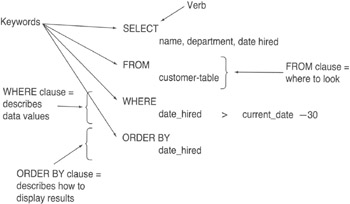
Figure 35.1: Basic structure of an SQL statement

As shown in Figure 35.1, each SQL statement begins with a keyword that describes what the statement does. Keywords you'll find at the beginning of SQL statements include: SELECT, INSERT, UPDATE, DELETE, CREATE, or DROP. After you tell the DBMS what you want done, you tell it the columns of interest and the table(s) in which to look. You normally identify the columns and tables you want to use by listing the columns after the verb (at the start of the SQL statement) and by listing the table(s) after the keyword FROM.

After you tell the DBMS what to do and identify the columns and tables to which to do it, you finish the SQL statement with one or more clauses that either further describe the action the DBMS is to take, or give a description of the data values that identify tables rows on which you want you want to DBMS to act. Typical descriptive clauses begin with the keywords: HAVING, IN, INTO, LIKE, ORDER BY, WHENEVER, WHERE, or WITH.

ANSI/ISO SQL-92 has approximately 300 reserved words of which you will probably use about 30 to do the majority of your work with the database. Table 35.1 lists some of the most commonly used keywords. Although some of the keywords are applicable only to MS-SQL Server, you will find keywords that perform similar functions if you are using another vendor's DBMS.

Table 35.1: Commonly Used SQL and MS-SQL Server Keywords

Keyword	Description
Data Definition Language (DML)
CREATE DATABASE	(MS-SQL Server). Creates a database and transaction log. A database has one or more schemas, which contain database objects such as tables, views, domains, constraints, procedures, triggers, and so on.
DROP DATABASE	(MS-SQL Server). Erases a database and transaction log.
CREATE SCHEMA	Adds a named container of database objects to the database. A database may have more than one schema. All database objects (tables, views, domains, constrains, procedures, triggers, and so on) reside in one of the schemas within the database.
DROP SCHEMA	Removes a schema from a database.
CREATE DOMAIN	Creates a named list of allowable values for columns in database tables. You can use domains as data types for columns in multiple tables.
DROP DOMAIN	Removes a domain definition from the database.
CREATE TABLE	Creates a structure (table) of columns and rows to hold data.
ALTER TABLE	Adds columns to a table, removes columns from a table, changes column data types, or adds column constraints to a table.
DROP TABLE	Removes a table from the database.
CREATE VIEW	Creates a database object that displays rows of one or more columns from one or more tables. Some views allow you to update the base tables.
DROP VIEW	Drops a database view.
CREATE INDEX	Creates a structure with values from a table column, which speeds up the DBMS's ability to find specific rows within the table.
DROP INDEX	Removes an INDEX from the database.
Data Manipulation Language (DML)
INSERT	Adds one or more rows to a table.
SELECT	Retrieves database data.
UPDATE	Updates data values in a table.
DELETE	Removes one or more rows from a table.
TRUNCATE	(MS-SQL Server). Removes all rows from a table.
Data Control Language (DCL)
ROLLBACK	Undoes changes made to database objects, up to the last COMMIT or SAVEPOINT.
COMMIT	Makes proposed changes to the database permanent. (COMMITTED changes cannot be undone with a ROLLBACK.)
SAVEPOINT	Marks points in a transaction (set of actions) that can be used to ROLLBACK (or undo) a part of a transaction without having to undo the entire transaction.
GRANT	Gives access to database objects or SQL statements.
REVOKE	Removes access privileges to database objects or executes specific SQL statements.
Programmatic SQL
DECLARE	Reserves server resources for use by a cursor.
OPEN	Creates a cursor and fills it with data values selected from columns in one or more rows in one or more database tables.
FETCH	Passes data values from a cursor to host variables.
CLOSE	Releases the resources used to hold the data copied from the database into a cursor.
DEALLOCATE	Releases server resources reserved for use by a cursor.
CREATE PROCEDURE	(MS-SQL Server). Creates a named list of SQL statements that a user (with the correct access rights) can execute by using the name as he or she would any other SQL keyboard.
ALTER PROCEDURE	(MS-SQL Server). Changes the sequence of SQL statements that the DBMS will perform when the user calls a procedure.
DROP PROCEDURE	(MS-SQL Server). Removes a procedure from the database.
CREATE TRIGGER	(MS-SQL Server, DB2, PL/SQL). Creates a named sequence of SQL statements that the DBMS will execute automatically when a column has a specific data value or when a user attempts a specific database command (the triggering event).
ALTER TRIGGER	(MS-SQL Server, DB2, PL/SQL). Changes the SQL statements executed when the DBMS detects the triggering event, or changes the nature of the event.
DROP TRIGGER	(MS-SQL Server, DB2, PL/SQL). Removes a trigger from the database.
DESCRIBE INPUT	Reserves an input area an application program will use to pass values to the DBMS during a dynamic SQL statement.
GET DESCRIPTOR	Tells the DBMS to use the DESCRIPTOR area to retrieve data values placed there by an application program during a dynamic SQL statement.
DESCRIBE OUTPUT	Reserves an output area the DBMS will use to pass data from the database to an application program during a dynamic SQL statement.
SET DESCRIPTOR	Tells the DBMS to place data into the DESCRIPTOR area for retrieval by an application program during a dynamic SQL statement.
PREPARE	Tells the DBMS to create an execution plan or compile the SQL statement(s) in a dynamic SQL statement.
EXECUTE	Tells the DBMS to execute a dynamic SQL statement.

You will find several tips on each of the common SQL statements (and others that are important, though not commonly used), throughout this book. The important thing to know now is that all SQL statements begin with a keyword (verb), have a list of objects on which to act, and may have one or more clauses that further describe the action or identify the rows on which to act at the end of the statement. If the SQL statement does not contain clauses that limit the action to rows with specific column data values, the DBMS will take action on all of the rows in a table (or multiples tables through a VIEW).

Understanding How the DBMS Executes SQL Statements

When processing an SQL statement, the DBMS goes through five steps:

• Parse. The DBMS goes through the SQL statement word by word and clause by clause to make sure that all of the keywords are valid and all of the clauses are well-formed. The DBMS will catch any syntax errors (badly formed SQL expressions) or typographical errors (misspelled keywords) during the parsing stage.
• Validate. The DBMS will check to make sure that all tables and columns named in the statement exist in the system catalog, as well as make sure there are no ambiguous column name references. During the validation step, the DBMS will catch any semantic errors (invalid references or valid references to nonexistent objects) and access violations (attempts to access database objects or attempts to execute SQL statements to which the user does not have sufficient privilege).
• Optimize. The DBMS runs an optimizer to decide on the best way to carry out the SQL statement. For a SELECT statement, for example, the optimizer checks to see if it can use an INDEX to speed up the query. If the query involves multiple tables, the optimizer decides if it should join the tables first and then apply the search condition, or vice versa. When the query appears to involve a scan of all rows in the table, the optimizers determines if there is a way to limit the data set to a subset of the rows in order to avoid a full table scan. Once the optimizer runs through all of the possibilities and gives them a rating based on speed (efficiency) and safety, the DBMS chooses one of them.
• Generate execution plan. The DBMS generates a binary representation of the steps involved in carrying out the SQL statement based on the optimization method suggested by the optimizer. The execution plan is what is stored when you create an MS-SQL Server procedure and what is generated when you prepare a dynamic SQL query. Generating the execution plan is the DBMS equivalent of compiling an application program to produce the .EXE file (the executable code).
• Execute. The DBMS carries out the action specified by the SQL statement by executing the binary execution plan.

Different steps in the process put different loads on the DBMS and server CPU. The parsing requires no database access and very little CPU time. Validation requires some database access but does not put too much of a load on the DBMS. The optimization step, however, requires a lot of database access and CPU time. In order to optimize a complex, multi-table query, for example, the optimizer may explore more than 20 ways to execute the statement.

The reason you don't just skip the optimization step is because the "cost" of doing the optimization is typically much less than the cost of performing the SQL statement in less than the most efficient manner. To put it another way, the reduction in time it takes to complete a well-optimized query more than makes up for the time spent in optimizing the query. Moreover, the more complex the query, the greater the benefits of optimization.

One of the major benefits of using procedures is being able to avoid performing the same parsing, validation, and (especially) optimization steps over and over again. When you enter an SQL query using an interactive tool (such as the MS-SQL Server Query Analyzer), the DBMS has no choice but to go through the entire five-step execution processor, even if you type in the same query multiple times.

If you put your SQL statement (or statements) into a stored procedure, however, the DBMS can parse, validate, optimize, and develop the execution plan in advance. Then, when you call the procedure, the DBMS needs only to execute the already compiled execution plan. Precompiled procedures let the DBMS avoid the "expensive" optimization phase the second and subsequent times you execute the SQL statements in the procedure. Thus, procedures let you move the first four steps of the execution process to the development environment, which reduces the load on the online production DBMS (and server).

Understanding SQL Keywords

SQL keywords are words that have a special significance in SQL and should not be used as user-defined names for database objects such as tables, columns, domains, constraints, procedures, variables, and so on. There are two types of keywords, reserved and nonreserved. The difference between reserved and nonreserved keywords is that some database products let you (although you should not) use nonreserved keywords to name database objects and variables. To make your SQL statements portable and less confusing, avoid using reserved words as identifiers.

When writing SQL statements, use all capital letters for keywords and lowercase letters for nonkeywords (or vice versa). Keywords are case-insensitive, meaning that the DBMS will recognize a keyword whether you type it using all capital letters, lowercase letters, or a combination of both. Making the case (capital vs. lower case) of reserved words different than non-reserved words in SQL statements makes the SQL statements easier for you (and those responsible for maintaining your database creation) to read.

Since each DBMS product supports most SQL-92 reserved words and adds a few of its own, the system manual and online help system are your best source for a list of reserved words. For example, to review MS-SQL Server's list of reserved words, perform the following steps:

1. Click on the Start button. Windows will display the Start menu.
2. Select Programs, Microsoft SQL Server 7.0 option, and click on Books Online. Windows will start the MS-SQL Server Help system.
3. Click on the Index tab and enter KEYWORDS in the Type in the Keyword to Find field. The MS-SQL Server Help system will display an alphabetical list of terms starting with Keywords.
4. To see a list of reserved keywords, click on Reserved and then click on the DISPLAY button. The Help system will display a dialog box asking you to select the type of reserved words on which you want its assistance.
5. Click on Reserved Keywords (T-SQL) and then click on the DISPLAY button. The MS-SQL Server Help system will display a list of T-SQL (Transact-SQL) reserved words, followed by a list of ODBC reserved words. The ODBC reserved words include the SQL-92 reserved words that MS-SQL Server supports. (Transact-SQL is MS-SQL Server's own procedural SQL language; Oracle uses PL/SQL and SQL Plus*.)

To exit the Help system, click on the close button (the X) in the upper-right corner of the Help application window.

Using the MS SQL Server Query Analyzer to Execute SQL Statements

You can use the MS-SQL Server Query Analyzer (QA) to execute any SQL statement supported by MS-SQL Server. (As mentioned in previous tips, no commercially available database supports everything in the SQL-92 standard.) QA has a graphical user interface (GUI) you can use to pose ad hoc (interactive) queries and to send SQL commands to an MS-SQL Server. (MS-SQL Server also provides a command-line interface to the database through ISQL, which you will learn about in Tip 39, "Using the MS-SQL Server ISQL to Execute SQL Statements from the Command Line or Statements Stored in an ASCII File.")

Note 

You will need to install MS-SQL Server prior to using the Query Analyzer. Tip 527 gives you step-by-step instructions for installing MS-SQL Server, if you have not yet installed it on your computer system.

To start to start MS-SQL Server QA, perform the following steps:

1. Click on the Start button. Windows will display the Start menu.
2. Select Programs, Microsoft SQL Server 7.0 option; click on Query Analyzer. Windows will start QA and display a Connect to SQL Server dialog box similar to that shown in Figure 38.1.

   
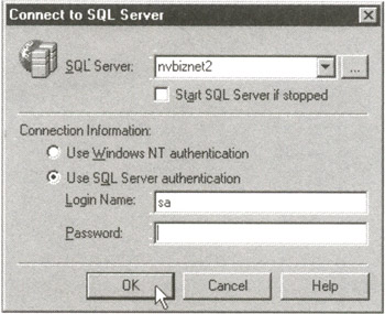
   Figure 38.1: MS-SQL Server Query Analyzer, Connect to SQL Server dialog box

3. Enter the name of the SQL Server to which you wish to connect in the SQL Server field. (The name of the SQL Server is typically the same as the name of the Windows NT Server on which you installed the MS-SQL Server.)
4. Enter your login name in the Login Name field. When you install MS-SQL Server, the program automatically creates the sa (system administrator) account without a password. If you are working with your own installed copy of the MS-SQL Server, use the sa account; if not, enter the Login Name and Password your system administrator (or database administrator) assigned to you.
5. Click on the OK button. QA will log in to the MS-SQL Server you specified in Step 4 and display the Query pane in the QA application window, similar to that shown in Figure 38.2.

   
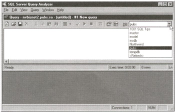
   Figure 38.2: The MS-SQL Server Query Analyzer Query pane in the Query Analyzer window

When you install MS-SQL Server under Windows NT, the installation program creates several databases, as shown in the DB drop-down list in the right corner of the Query pane in Figure 38.2. Before using QA to send SQL statements to the MS-SQL Server, you must select a database.

To work with the pubs (sample) database, perform the following steps:

1. Click on the drop-down button to the right of the DB field (in the upper-right corner of the QA Query pane) to list the databases on the SQL Server to which you are connected.
2. Click on a database to select it. For the current example, click on pubs.
3. Place your cursor in the Query pane by clicking anywhere within it. QA will place the cursor in the upper-left corner of the Query pane.
4. Enter your SQL statement in the Query pane. For the current example, enter SELECT * FROM authors.
5. To execute the query (entered in Step 4), either press F5 or Ctrl+E, or select the Query menu Execute option. For the current example, press F5. QA will display your query results in a Results pane below the Query pane, similar to that shown in Figure 38.3.

   
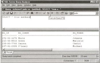
   Figure 38.3: The Query Analyzer, with a query in the Query pane and query results in a Results pane

Whenever you tell QA to execute the SQL in the Query pane, QA will send all of the statements in the Query pane to the SQL Server for processing, unless you select a specific statement (or set of statements) you want to execute. So, be careful you don't press Ctrl+E (or press F5, or select the Query menu Execute option), thinking that QA will send only the last statement you typed to the SQL server.

If you have multiple statements in the Query pane, either remove the ones you don't want to execute, or highlight the statement(s) that you want QA to send to the SQL Server for processing. For example, if you, you had the following statements in the Query pane

SELECT * FROM authors
SELECT * FROM authors WHERE au_lname = 'Green'

and you only wanted to execute the second statement, highlight the second query to select it and then select the Query menu Execute option (or click on the green Execute Query button on the standard toolbar). QA will send only the second select statement to the SQL Server and display the results in the Results pane, similar to that shown in Figure 38.4.

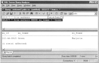
Figure 38.4: The Query Analyzer after executing the highlight statement when the Query pane contains multiple statements

Having QA retain SQL statements in the Query pane after it executes them can save you a lot of typing, especially if you enter a complex query and don't get the results you expect. If you need to change the logic of your query's selection clause, you need only click your cursor in the SQL statement and make your change, without having to retype the entire statement.

Using the MS SQL Server ISQL to Execute SQL Statements from the Command Line or Statements Stored in an ASCII File

In Tip 38, "Using the MS-SQL Server Query Analyzer to Execute SQL Statements," you learned how to use the MS-SQL Query Analyzer GUI query tool. MS-SQL Server also includes two command-line query tools: ISQL.EXE and OSQL.EXE. You'll find both of these tools in MS-SQL Server's BINN subdirectory. (If you installed MS-SQL Server to the default C:MSSQL7 folder, you will find ISQL and OSQL in the C:MSSQL7BINN sub-folder.)

Aside from the name, the only difference between ISQL and OSQL is that ISQL uses DB-LIB to connect to the database, whereas OSQL uses ODBC. Although we'll use ISQL to access that database in this tip, the important thing to know is that you can execute the same statements using OSQL. Thus, if you have only OSQL on your system, just use it in place of ISQL in the following example.

The command-line query tools are useful if you find yourself running a series of SQL statements. You can use ISQL (or OSQL) to execute the statements one after another by typing them into an ASCII that you pass to ISQL or OSQL for processing. The command-line tools also give you a quick, low overhead way to test your SQL queries.

Note 

You will need to install MS-SQL Server prior to using either of the two command-line query tools (ISQL or OSQL). Tip 527 gives you step-by-step instructions for installing MS-SQL Server, if you have not yet installed it on your computer system.

If you are using the computer on which you installed MS-SQL Server, you need type only I SQL or OSQL at the MS-DOS prompt to start the query tool because the installation program added the C:MSSQL7BINN folder in your path. If you are attaching to the MS-SQL Server across a network, have your system administrator give you access to the MSSQL7BINNOSQL.EXE on the server. (In order to use ISQL.EXE, you must install NTWDBLIB.DLL on your computer—OSQL.EXE does not require an additional DLL file.)

Before you can start using ISQL, you must get to an MS-DOS prompt. If you have an MS-DOS icon on your desktop, double-click on it. Otherwise, click your mouse on the Start button, select Programs, and then click your mouse on Command Prompt. Windows will start an MS-DOS session.

The format of the command to start ISQL is:

ISQL -S -U -P

(If you want to see the list of all ISQL command line parameters, type ISQL-? and then press the Enter key.)

To use ISQL to attach to your MS-SQL Server, replace with the name of your MS-SQL Server, and replace and with your login name and password. For example, to attach to the MS-SQL Server NVBizNet2 using the login name sa, which has no password, type

ISQL -SNVBizNet2 -Usa -P

and then press the Enter key. ISQL will display its equivalent of the MS-DOS prompt, similar to that shown in Figure 39.1.

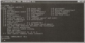
Figure 39.1: The ISQL response to the - ? parameter, followed by the ISQL Ready prompt (1>) after ISQL successfully attached to the NVBizNet2 SQL Server

Once you see the ISQL Ready prompt, perform the following steps to send SQL statements to the SQL server:

1. Type an SQL statement at the Ready (1>) prompt. For the current example, type USE pubs (to tell the SQL Server you want to use the PUBS database), and then press the Enter key. ISQL will respond with the Ready prompt 2>, indicating that it is ready for you to enter the second line of commands.
2. Type an SQL statement. For the current example, type SELECT * FROM authors WHERE zip = 94609 and then press the Enter key. ISQL will respond with the Ready prompt 3>, waiting for the third statement or command.
3. If you have additional statements you want ISQL to send to the server as a group, repeat Step 2 until you finish entering.
4. Type GO and the press the Enter key to tell ISQL to send your SQL statements to the SQL server.

After you complete Step 4, ISQL will send the SQL statements you entered prior to the GO command to the DBMS, display the results, and then indicate that it is ready for your next command by displaying another Ready prompt (1>).

The important thing to understand is that ISQL sends your SQL statements to the SQL Server only after you type GO at a ready prompt and press the Enter key.

To exit ISQL, type EXIT at a ready prompt and then press the Enter key. ISQL will terminate and your computer will return to the MS-DOS prompt.

To exit your MS-DOS session and return to the Windows desktop, type EXIT at the MS-DOS prompt and press the Enter key.

Note 

By typing USE pubs in Step 2, you told the DBMS that you wanted to use the PUBS database. Instead of having ISQL send the USE statement to the DBMS, you can select the database you want to use by adding -d when you start ISQL. In the current example, you would have entered:

ISQL -SNVBizNet2 -Usa -P -dpubs

To start ISQL, log in to the sa account on the NVBizNet2 SQL Server and select PUBS as the database to use in subsequent SQL statements.

As mentioned at the beginning of this tip, you can type SQL statements into an ASCII file and then have ISQL (or OSQL) execute them. To do so, add the -i parameter when typing the ISQL startup command. Suppose, for example, that you had the following statements in a file named INFILE39.SQL:

USE pubs
SELECT au_ID, au_lname, zip FROM authors WHERE zip = 94301
GO

You could tell ISQL to send the two statements in INFILE39.SQL to the DBMS and display the results to the screen by starting ISQL with the command line:

ISQL -SNVBizNet2 -Usa -P -dpubs -iInFile39.sql -n

The -n tells ISQL not to display statement numbers. Without the -n, ISQL will display a statement number and the greater than (>) symbol for each of the three SQL statements. As a result, the headings won't line up with the column data. The -n tells ISQL not to display the statement line numbers. After you enter the command line, press the Enter key. ISQL will send each of the statements in the input file InFile39.sql to the DBMS and display output similar to:

 au_ID au_lname zip
 ----------- ------------ ----
 427-17-2319 Dull 94301
 846-92-7186 Hunter 94301

As a final permutation, to store the query results in a file instead of displaying them to the screen, add the -o parameter to the ISQL startup command. Suppose, for example, that you want to store the query results from executing the statements in the input INFILE39.SQL into the output file OUTFLE39. You would type

 ISQL -SNVBizNet2 -Usa -P -iInFile39.sql -n -oOutFle39

at the MS-DOS prompt and then press the Enter key to start ISQL.

Using the ED Command Within ISQL to Edit SQL Statements

Before sending SQL statements to the DBMS when you enter the GO command, ISQL acts as a line editor. As you learned in Tip 39, "Using the MS-SQL Server ISQL to Execute SQL Statements from the Command Line or Statements Stored in an ASCII File," the format of the command to start ISQL at the MS-DOS command line is:

ISQL -S -U -P

Note 

Substitute the name of your SQL Server for NVBizNet2, and use your own username and password for login if the sa account is not available to you.

Thus, to log in to the NVBizNet2 MS-SQL Server as username sa, perform the following steps:

1. Click your mouse on the Start button, select Programs, and click your mouse on Command Prompt. Windows will start an MS-DOS session.
2. To start ISQL, type ISQL -SNVBizNet2 -Usa -P and press the Enter key. ISQL will display its Ready prompt (1>).
3. Next, enter the SQL SELECT statement:

   SELECT * FROM authors
   

4. Press the Enter key. After ISQL puts your statement in its statement buffer, your screen will appear similar to the following:

   ISQL -SNVBizNet2 -Usa -P
   1> SELECT * FROM authors
   2>
   

Since you did not identify the database you want to use, ISQL will display the following if you enter GO and press the Enter key at the Ready prompt (2>).

 Msg 208, Level 16, State 1, Server NVBIZNET2, Line 1
 Invalid object name 'authors'.

Because ISQL is a line editor interface, you cannot move your cursor in front of SELECT and insert a statement. Thus, if you had only ISQL, your only choice would be to enter EXIT or QUIT at the Ready prompt (2>) and start over, this time either adding the -d parameter to the ISQL command line or typing USE in response the first Ready prompt (1>).

Fortunately, ISQL lets you use the MS-DOS full-screen editor.

To start the full screen editor, type ED at a ready prompt (2>) and press the Enter key. ISQL will start the MS-DOS editor and transfer the contents of its statement buffer, similar to that shown in Figure 40.1.

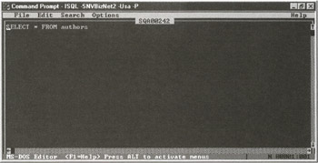
Figure 40.1: The MS-DOS full-screen editor as started by ISQL

To insert the USE statement in front of the SELECT statement, move your cursor in front of the word SELECT. Type USE pubs and press the Enter key. Once you've done that, you will have two statements in the text editor:

 USE pubs
 SELECT * FROM authors

To transfer the contents of the full-screen editor to the ISQL statement buffer, select the File, Exit option. When the editor prompts you to save your changes, press Y. The MS-DOS editor will send its contents to ISQL which will display them as individual lines similar to:

 1> USE pubs
 2> SELECT * FROM authors
 3>

Now, type GO and press the Enter key to send the USE and SELECT statements to the DBMS. After ISQL displays the query results, type EXIT and press the Enter key to exit ISQL and return to the MS-DOS prompt.

The important things to know are:

• You can work in single-line edit mode by typing your SQL statements in response to each ISQL Ready prompt.
• ISQL stores each statement you enter in its statement buffer.
• You can use a full-screen editor by entering ED in response to an ISQL Ready prompt.
• When you start the full-screen editor (with the ED command), ISQL copies the contents of its statement buffer to the editor screen.
• When you leave the full-screen editor (by selecting the File menu Exit option), ISQL reads the contents of the editor screen into its statement buffer as one statement per editor line.

Using the CREATE DATABASE Statement to Create an MS SQL Server Database and Transaction Log

Unlike many other DBMS products, MS-SQL Server lets you create multiple databases for each MS-SQL Server. Most commercial DBMS products do not even have a CREATE DATABASE command. Instead, the installation program creates the one database file the SQL Server will use. The database administrator (dba) and privileged users then create all of the database objects in the one database. As a result, the typical database contains a mix of both related and unrelated tables.

MS-SQL Server gives you the best of both worlds. If you want, you can create a single database for all of your tables, or you can separate totally unrelated tables into separate databases. Suppose, for example, that you and your spouse each run your own home business. Using the typical DBMS, you would create one database to hold both your (mail order) CUSTOMER list and your spouse's (accounting) CLIENT list, even though the two tables are completely unrelated.

Having a single database means that both businesses would lose database access during backup and (if necessary) recovery operations. If the two were separate, you could still use a single server (to save a bit of hard-earned cash on software and hardware), but you would not be affected by database problems or maintenance activities that have nothing to do with your own tables.

Finally, MS-SQL Server's multiple database strategy makes it possible to create a development database that uses the same database objects and security setup as its production counterpart. Having an identical database structure and security setup makes it easier to test how proposed changes will affect online application programs, database stored procedures, views, and triggers. Moreover, once you've fully tested new or modified code on the development system, you will be able to install procedures, triggers, and views on the production system without further modification. Finally, you can import data from tables in the production database into identical tables in the development database, making it easy to use the development system to "freeze" database data and reproduce errors that seem to occur at random intervals.

The syntax of the CREATE DATABASE statement is:

 CREATE DATABASE 
 [ON {[PRIMARY] } [,...]]
 [LOG ON { } [,...]]
 [FOR RESTORE]
  is defined as:
 (NAME = ,
 FILENAME = ''
 [, SIZE = ]
 [, MAXSIZE = { | UNLIMITED}]
 [, FILEGROWTH = ])

Review Table 41.1 for a brief explanation of CREATE DATABASE keywords and options.

Table 41.1: Definition of CREATE DATABASE Statement Keywords and Options

Keyword/Option	Description
database name	The name of the database.
ON	The name(s) of the disk file(s) that will hold the data portion of the database. MS-SQL Server lets you split a single database into multiple files.
PRIMARY	If you split the database into multiple files, PRIMARY identifies the file that contains the start of the data and the system tables. If you don't specify a PRIMARY file, MS-SQL Server will use the first file in the list as the PRIMARY file.
LOG ON	The name(s) of the disk file(s) that will hold the transaction log.
FOR RESTORE	Do not allow access to the database until it is filled with data by a RESTORE operation.
	The name the MS-SQL Server will use to reference the database or transaction log.
	The full pathname to the database or transaction log file.
	The initial size, in megabytes, of the database or transaction log. If you don't specify an initial size for the transaction log, the system will size it to 25 percent of the total size of the database files.
	The maximum size to which the database or transaction log can grow. If you specify UNLIMITED, the files can grow until they exhaust the physical disk space.
	The number of bytes to add to the size of the transaction log or database file when the current free space in the file is used up.

To create a database using the MS-SQL Server Query Analyzer, perform the following steps:

1. Click your mouse on the Start button. Windows will display the Start menu.
2. Move your mouse pointer to Programs on the Start menu, select the Microsoft SQL Server 7.0 option, and click your mouse on Query Analyzer. Query Analyzer will display the Connect to SQL Server dialog box similar to that shown in Figure 41.1.

   
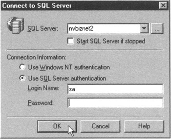
   Figure 41.1: The Query Analyzer Connect to SQL Server dialog box

3. Enter the name of your SQL Server in the SQL Server field.
4. Enter your username in the Login Name field, and enter your password in the Password field.
5. Click on the OK button. Query Analyzer will connect to the SQL Server you entered in Step 3 and display the Query pane in the SQL Server Query Analyzer application window.
6. Enter the CREATE DATABASE statement. For the current example, enter:

   CREATE DATABASE SQLTips
   ON (NAME = SQLTips_data,
    FILENAME = 'c:mssql7dataSQLTips_data.mdf',
    SIZE = 10,
    FILEGROWTH = 1MB)
   LOG ON (NAME = 'SQLTips_log',
    FILENAME = 'c:mssql7dataSQLTips_log.ldf',
    SIZE = 3,
    FILEGROWTH = 1MB)
   

7. Click on the green arrow Execute Query button on the standard toolbar (or select the Query menu Execute option). Query Analyzer will create the database on the SQL Server to which you connected in Step 5.

After you complete Step 7, the Query Analyzer will display the results of the CREATE DATABASE execution in the Results pane in the SQL Server Query Analyzer application window. If Query Analyzer is successful in executing your CREATE DATABASE statement, the program will display the following in the Results pane:

 The CREATE DATABASE process is allocating 10.00 MB on disk 'SQLTips_data'.
 The CREATE DATABASE process is allocating 3.00 MB on disk "SQLTips_log'.

Using the MS SQL Server Enterprise Manager to Create a Database and Transaction Log

In Tip 41, "Using the CREATE DATABASE Statement to Create an MS-SQL Server Database and Transaction Log," you learned that MS-SQL Server lets you create multiple databases on a single server, and you also learned how to use the CREATE DATABASE statement. Like most database management tools, MS-SQL Server gives you not only a command line (SQL or Transact-SQL) statement, but also a graphical user interface (GUI) tool to perform the same function. To create a database using the MS-SQL Server Enterprise Manager, perform the following steps:

1. Click your mouse on the Start button. Windows will display the Start menu.
2. Move your mouse pointer to Programs on the Start menu, select the Microsoft SQL Server 7.0 option, and click your mouse on Enterprise Manager. Windows will start the Enterprise Manager in the SQL Server Enterprise Manager application window.
3. Click your mouse on the plus (+) to the left of SQL Server Group to display the list of MS-SQL Servers available on your network.
4. Click your mouse on the plus (+) to the left of the SQL Server on which you wish to create a database. Enterprise Manager, in turn, will display a Database Properties dialog box similar to that shown in Figure 42.2
5. Click your mouse on the Databases folder to display the list of databases currently on the server, similar to that shown in Figure 42.1.

   
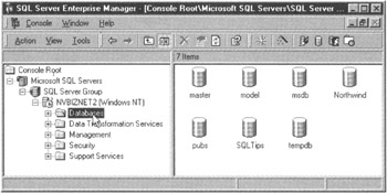
   Figure 42.1: The SQL Server Enterprise Manager application window

6. Select the Action menu New Database option. Enterprise Manager displays a Database Properties dialog box similar to that shown in Figure 42.2.

   
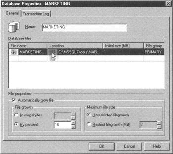
   Figure 42.2: The Enterprise Manager Database Properties dialog box

7. Enter the name of the database in the Name field. For the current project, enter MARKETING. The Enterprise Manager will automatically fill in the pathname and initial database size in the Database Files section of the Database Properties dialog box.

   Note 

   If you want to put the database in a folder other than the default folder or change the physical file name, click your mouse on the Search button in the Location field in the Database Files area of the Database Properties dialog box. Enterprise Manager will display the Locate Database File dialog box so you can select a folder or change the database's physical file name.

8. Click on the Initial size (MB) field and enter the initial size of the database file. For the current project, enter 10.
9. Set the database File Growth and Maximum File Size options. For the current project, accept the defaults, which allow the database file to grow by 10 percent each time it fills up and place no restriction on its maximum size.
10. Click on the Transaction Log tab.
11. If you want to change the pathname (the file name and physical location) of the transaction log file, click on the Search button in the Location field to work with the Locate Transaction Log File dialog box. For the current project, accept the default pathname for the transaction log.
12. Click on the Initial size (MB) field, and enter the initial size of the transaction log. For the current project, enter 3.
13. Set the database File Growth and Maximum File Size options. For the current project, accept the defaults, which allow the transaction log to grow by 10 percent each time it fills up and place no restriction on its maximum size.
14. Click on the OK button.

After you complete Step 14, the Enterprise Manager will create the database (MARKETING, in the current example) according to the options you selected and return to the SQL Server Enterprise Manager application window.

The important thing to know now is that MS-SQL Server gives you two ways to create a database. You can use the CREATE DATABASE statement or use the Enterprise Manager's Action menu New Database option. Whether you use CREATE DATABASE or the Enterprise Manager, you can set database and transaction log options that specify:

• The physical locations (pathnames) of the database and transaction log file(s)
• The initial size of the database and transaction log
• The increment by which the database and transaction log will grow
• The maximum size to which the database and transaction log file(s) can grow

If you are using CREATE DATABASE, you specify the database and transaction log properties in separate clauses within the statement. When you use the Enterprise Manager to create a database, you can still specify different properties for the database and transaction log file(s) by using the Database Properties dialog box General tab to specify database options and using the Transaction Log tab to select transaction log options.

Using DROP DATABASE to Erase an MS SQL Server Database and Transaction Log

Dropping (deleting) databases you no longer need frees up disk space. The primary rule to follow: Be careful! You cannot easily undo an executed DROP DATABASE statement. As such, always back up the database before dropping (erasing) it. Having a full backup will save you a lot of headaches if the user decides he or she needs "one more thing" from the database-right after you erase it, of course.

Only the system administrator (sa) or a user with dbcreator or sysadmin privilege can drop a database. You cannot drop the MASTER, MODEL, or TempDB database.

The syntax of the DROP DATABASE statement is:

DROP DATABASE 
 [,, ]

Thus, to remove the MARKETING database you created in Tip 42, "Using the MS-SQL Server Enterprise Manager to Create a Database and Transaction Log," perform the following steps:

1. Start the MS-SQL Server Query Analyzer (as you learned to do in Tip 38, "Using the MS-SQL Server Query Analyzer to Execute SQL Statements"), or start the Enterprise Manager (as you learned to do in Tip 42) and select the Tools menu, SQL Server Query Analyzer option.
2. Enter the DROP DATABASE statement in the Query Analyzer's Query pane. For the current project, type

   DROP DATABASE marketing.
   

3. Press Ctrl+E (or select the Query menu, Execute option).

   After you complete Step 3, the Query Analyzer will attempt to delete the database and log file. If Query Analyzer successfully deletes the MARKETING database and transaction log, it will display the following in the Results pane of the Query Analyzer application window:

    Deleting database file 'C:MSSQL7dataMARKETING_Data.MDF'.
    Deleting database file 'C:MSSQL7dataMARKETING_Log.LDF'.
   

Understanding How to Size MS SQL Server Databases and Transaction Logs

MS-SQL Server puts all database objects (tables, views, procedures, triggers, indexes, and so on) into a single large file. Whenever you make a change to the database (add an object, alter an object, delete a row, update a column value, insert a row, and so on), the DBMS makes an entry in a second file, the transaction log. Thus, every database has two files: the database file, which contains all of the database objects; and the transaction log, which contains an entry for each change made to the database (since the last time the log was cleared).

Note 

The database file and transaction log can each be made up of more than one physical file. However, the DBMS treats the set of physical files used to hold the database data as a single, logical "database file" and the set of physical files used to hold the transaction log as a single, logical "transaction log" file. You can set the initial size of each individual file, but the FILEGROWTH option applies to the logical database file and transaction log, not to each physical file used to store them on disk.

As you learned in Tip 41, "Using the CREATE DATABASE Statement to Create an MS-SQL Server Database and Transaction Log," and Tip 42, "Using the MS-SQL Server Enterprise Manager to Create a Database and Transaction Log," you use the SIZE option to specify the initial size of the database and transaction log when you create them. For example, in Tip 41, you executed the SQL statement

CREATE DATABASE SQLTips
ON (NAME = SQLTips_data,
 FILENAME = 'c:mssql7dataSQLTips_data.mdf',
 SIZE = 10,
 FILEGROWTH = 1MB)
LOG ON (NAME = 'SQLTips_log',
 FILENAME = 'c:mssql7dataSQLTips_log.ldf',
 SIZE = 3,
 FILEGROWTH = 1MB)

which created the SQLTips database file (SQLTIPS_DATA.MDF) with an initial size of 10MB and the transaction log for the database (SQLTIPS_LOG.LDF) with an initial size of 3MB. As you add rows to tables in the database, you use up the free space in the database file. If you add data to a table where each row consists of 10 columns of type CHAR(100), you use up 1,000 bytes (10 columns X 100 bytes / column) of the 10MB available each time you add a row to the table.

Once you've used all of the free space in a database file (10MB, in the current example) you can no longer add data to the database, even if there is a large amount of physical disk storage space available. To avoid running out of room in the database file before exhausting the physical disk space, use the FILEGROWTH option when you create a database. The FILE-GROWTH option tells MS-SQL Server to extend the size of the database file each time it gets full.

In the current example, you set FILEGROWTH to 1MB, which means that each time you use up the space allocated to the database file, the DBMS will increase the size of the file by 1MB. Moreover, since you did not specify a maximum database file size, the DBMS will extend the database file 1MB at a time (as necessary) until it exhausts the physically disk storage space.

Each time you make a change to the database, the DBMS stores the original data values and makes a notation detailing what was done in the transaction log. As such, the DBMS may use up the 3MB allocated to the transaction log in the current example rather quickly if you are making a lot of changes to the database. Fortunately, you can have MS-SQL Server extend the size of the transaction log, just as it does the size of the database file.

In the current example, the DBMS will add 1MB of free space to the transaction log each time the transaction log file fills up.

Note 

Although the current example uses the same FILEGROWTH value for the database file and the transaction log, the two are independent. For example, you can set the FILEGROWTH at 5MB for the database file and 3MB for the transaction log-one does not depend on the other.

Be sure to specify a large enough initial database file size and growth factor so that your DBMS isn't spending the majority of its time extending the size of the database file as you add table rows. To determine the initial database file size, perform the following analysis on each table in the database:

1. List the column name, data type, and number of bytes of disk space the DBMS will need to store a value in the column. (Your system manual will have a breakdown of the storage required for the data types your DBMS supports.)
2. Determine the number of rows you expect the table to hold within the first six months (or year) of operation.
3. Multiply the number of bytes per row times the number of rows in the table to determine the storage requirements of the table.

Once you know the storage required for each table in your database, set the initial size of the database file to 25-50 percent more than the sum of the space required by all of its tables. The extra space (50 percent, if possible), allows for a margin of error for your guess as to the number or rows you expect each table to hold, leaves space for indexes the DBMS can add to speed up data access, and gives the DBMS room for system cursors and for temporary tables it creates when processing complex queries with large result sets.

Set the FILEGROWTH option to 10 percent of the initial database file size, rounded up to the nearest whole number. Thus, if your initial database file size is 25MB, set your FILE-GROWTH to 3MB. Monitor the size of your database file, especially during the first several months of operation. If you find the database file growing at more than 10 percent in a month, increase the FILEGROWTH option so that the DBMS has to extend the database file size only once a month.

As a general rule of thumb, set the initial size of your transaction log file to 25 percent of the initial size of your database file, and set its FILEGROWTH to 10 percent of its initial size. Thus, if your initial database file size is 250MB, set the transaction log file to start at 25MB and grow by 3MB. Monitor the growth in size of your transaction log, and adjust its growth factor so that the DBMS has to extend it at most only once per month.

You learned how to set the initial file size and the growth increment (FILEGROWTH) for your database and transaction log files using the CREATE DATABASE statement in Tip 41 and using the MS-SQL Server Enterprise Explorer in Tip 42. After you've created the database file and transaction log, you can use the Enterprise Manager to change the size of either the file or its growth factor by performing the following steps:

1. To start the Enterprise Manager, click on the Start button, move your mouse pointer to Programs on the Start menu, select Microsoft SQL Server 7.0, and click your mouse on Enterprise Manager.
2. To display the list of SQL Servers, click on the plus (+) to the left of SQL Server Group.
3. To display the list of resources on the SQL Server with the database file or transaction log you want to modify, click on the plus (+) to the left of the SQL Server's name. For example, if you want to work with the SQL Server NVBizNet2, click on the plus (+) to the left of NVBizNet2. Enterprise Manager will display a list of folders that represent the resources managed by the SQL Server NVBizNet2 (in the current example).
4. Click on the Databases folder. The Enterprise Manager will display the databases on the SQL Server in its right pane.
5. Double-click your mouse on the database icon whose database file or transaction log you want to modify. For the current example, double-click your mouse on SQLTips (if you created the database in Tip 41). Enterprise Manager will display the General tab of the SQLTips Properties dialog box similar to that shown in Figure 44.1. (The name of the dialog box is Properties.) As such, your dialog box will be SQLTips Properties only if you double-clicked your mouse on the SQLTips database.

   
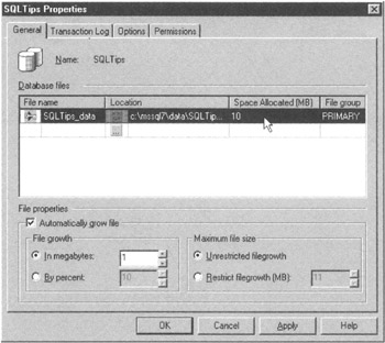
   Figure 44.1: The Enterprise Manager database properties dialog box

6. Click on the Space Allocated field in the Database files area of the dialog box. For the current example, change the 10 to 15.
7. To have the database file grow by a percentage of its current size instead of by a constant number of megabytes, click your mouse on the By Percent radio button in the File Properties area of the dialog box. For the current example, leave the percentage the default, 10 percent.
8. If you want to restrict the database file growth to a certain number of megabytes, click on the Restrict Filegrowth (MB) radio button and enter the maximum file size in megabytes. For the current example, allow for unrestricted file growth by clicking on the Unrestricted Filegrowth radio button.
9. Click on the Transaction Log tab to work with the transaction log properties. For the current example, leave the transaction log properties unchanged. However, if you did want to change the transaction log options, you would follow Steps 6 to 8, substituting "transaction log" for "database file" in each step.
10. Click on the OK button. The Enterprise Manager will apply your changes to the SQLTips database and return to the Enterprise Manager application window.

The optimal initial size and growth increment for a database and transaction log depend on the amount of data, amount of physical storage space available, and volume of transactions you expect the DBMS to handle. If you're converting from one DBMS product to another, base your size and increment settings on historical requirements. Otherwise, use the figures in this tip as a reasonable starting point. The important thing to understand is that while you don't want to allocate space you'll never need, you also want the DBMS to spend as little time as possible increasing the size of the database file and transaction log.

Understanding the MS SQL Server TempDB Database

Each time you start MS-SQL Server, the DBMS creates a special database named TempDB. The server uses the TempDB database for such things as temporary tables, cursor data, and temporary, user-created global variables. In short, the TempDB database is the system's scratchpad. However, you can use it as well.

The advantage of using TempDB is that activities you perform to TempDB objects (tables, views, indexes, and so on) are not logged. As such, the DBMS can manipulate data in TempDB faster than it does in other databases.

Prior to changing database objects and data values (other than TempDB objects and data), the DBMS must store the preupdate (original) object structures and values in the transaction log. Thus, for non-TempDB data, every data manipulation involves two save operations— save the original and then save the updated value. Saving the original data values can impose significant overhead if you are making a large number of changes. When using TempDB objects, however, the DBMS has to perform storage operations only once—to save the updated values to disk.

The downside of using TempDB objects is that you cannot roll back (or undo) manipulations made on TempDB objects. Moreover, each time you shut down the DBMS and restart it, TempDB (and all of its objects) is erased. As such, any information stored in TempDB is lost each time the DBMS restarts (and re-creates TempDB). Therefore, do not rely on the existence of any information in TempDB from one session to the next.

Use TempDB as a scratchpad (as MS-SQL Server does) to hold temporary data values and tables. TempDB is especially useful for aggregating data values from multiple tables in order to generate a summary report. Rather than trying to write an SQL statement that both selects and summarizes data, you can simplify your task by writing a query that aggregates the data you want in a temporary TempDB table, and then execute a simple second query to produce your final report.