Hack 72. Add Relief to Your Topographic Maps

Using GRASS and some digital elevation models, you can give existing topo maps a more expressive "3-D" look.

Topographic maps can be a useful tool for getting a sense of the lay of the land, but the contour lines used to express topographic variation can be a little hard to get one's head around at a glance. Does that path lead uphill or downhill? By adding shadows to the map that correspond to the contours of the land (as if the sun were overhead), we can create the impression of relief on our topo maps, making it easier for the eye to pick out hills and valleys. This technique is called hill shading, and GRASS offers several tools for adding hill shading to a topographic map.

6.10.1. Getting the Data

For simplicityand because there is a wealth of freely available data for the regionwe'll try our hand at adding hill shading to a topographic map of San Francisco. Hill shading involves not only a nice topo map, but also elevation data to plot the relief with. Fortunately, the USGS Bay Area Regional Database at http://bard.wr.usgs.gov/ offers both (and more!) for the San Francisco Bay Area. We'll start by downloading the data to make our relief map. Visit http://bard.wr.usgs.gov/htmldir/sf_100k.html and download the digital raster graphic (DRG) and the DRG world file for the San Francisco quadrangle. Then go to http://bard.wr.usgs.gov/htmldir/dem_html/dem10_mtr_sf.html and get the gzip-compresed digital elevation model (DEM) files for Point Bonita, San Francisco North, San Francisco South, San Francisco South West, Oakland West, and Hunter's Point. All told, you'll be downloading a bit less than 9 MB of compressed data.

Now we'll uncompress the data we just downloaded. If you put all of these files into a new directory, you can just run:

$ gunzip *.gz

This may take a few moments. Now we have 71 MB of uncompressed data. Let's run gdalinfo [Hack #68] , which is part of the GDAL package, on one of the DEM files, to see what projection they're in. If you don't already have GDAL installed, you can get it from Debian apt or download source code or binaries from http://gdal.maptools.org/. The output from gdalinfo looks like this:

$ gdalinfo sf_north.dem 
Driver: USGSDEM/USGS Optional ASCII DEM
Size is 1109, 1395
Coordinate System is:
PROJCS["UTM Zone 10, Northern Hemisphere",
 GEOGCS["NAD27",
 DATUM["North_American_Datum_1927",
 SPHEROID["Clarke 1866",6378206.4,294.978698213898,
 AUTHORITY["EPSG","7008"]],
 TOWGS84[-3,142,183,0,0,0,0],
 AUTHORITY["EPSG","6267"]],
 PRIMEM["Greenwich",0,
 AUTHORITY["EPSG","8901"]],
 UNIT["degree",0.0174532925199433,
 AUTHORITY["EPSG","9108"]],
 PROJECTION["Transverse_Mercator"],
 PARAMETER["latitude_of_origin",0],
 PARAMETER["central_meridian",-123],

That's quite a bit of metadata, but it tells us a few things we need to know in order to create a new location in GRASS. As usual, a lot of the USGS's freely available topographic data is stored in UTM coordinates, referenced to the NAD27 geodetic datum. (NAD27 has since been superseded by NAD83, but the USGS still has most of its data kicking about in NAD27.)

If you're outside the Bay Area, you might try getting National Elevation Data (NED) and other base maps from the USGS Seamless Data Distribution System [Hack #67] . Obviously, the smaller the resolution you can get, the better. For areas outside the U.S., you might try NASA's Shuttle Radar Topography Mission (SRTM) data, available from the Global Land Cover Facility at http://landcover.org/data/srtm/. In either event, you may need to [Hack #68] first.

 

6.10.2. Creating a New Location in GRASS

Start up GRASS, and create a new location using the UTM coordinate system. The NAD27 datum is based on the Clarke 1866 ellipsoid model, so select clark66 for your ellipsoid and nad27 for your map datum. San Francisco is in the Northern Hemisphere, in UTM zone 10. You can leave the extents at their defaults. Once you're back at the opening menu, load your new location. You should now be at the GRASS prompt.

Let's start by importing the digital raster graphic containing the topo map. Remember that DRG world file you downloaded? Sometimes GeoTIFF files keep their projection metadata stored in a separate world file. GRASS's raster import utility, r.in.gdal (so named for the GDAL raster data library it's based on) needs this file to figure out how your DRG is georeferenced, but, for whatever reason, it expects a different file extension, so we'll have to rename the world file before feeding the DRG to r.in.gdal. Then we'll import the topo map into a raster layer called sf_topo and view it on a graphics monitor. Since the DRG doesn't have any projection metadata attached, we'll have to tell r.in.glad that we know that the image is correct, by giving it the -o option to override the current GRASS projection:

GRASS:~/shade > mv sanfrancisco_ca.tiffw sanfrancisco_ca.tfw
GRASS:~/shade > r.in.gdal -o in=sanfrancisco_ca.tiff out=sf_topo
GRASS:~/shade > g.region raster=sf_topo
GRASS:~/shade > d.mon start=x0
using default visual which is TrueColor
ncolors: 16777216
Graphics driver [x0] started
GRASS:~/shade > d.rast sf_topo
 100%

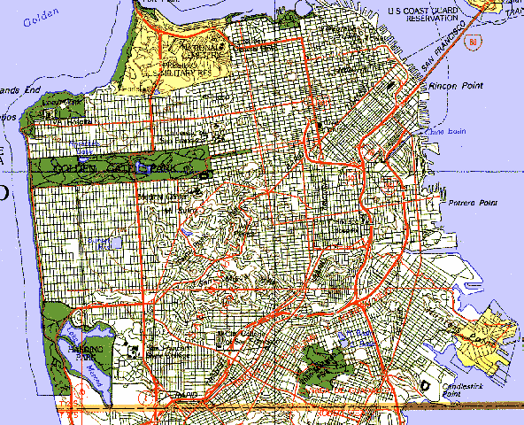
Voilà! Figure 6-34 shows a rather nice looking topo map of San Francisco and its surroundings, albeit from a distance. Use d.zoom to zoom in and get a feel for the contents of the topo map. If you zoom in all the way, you can see curved brown lines that represent the topographic contours. It's a bit hard to tell just from looking where the hills begin and end, isn't it?

Figure 6-34. The USGS DRG for San Francisco, imported into GRASS

In binary distributions of older versions of GRASS, r.in.gdal had an unfortunate tendency to segfault. If you're running one of these versions, try one of the other r.in functions, like r.in.tiff. If your data isn't already in GeoTIFF format, you can always [Hack #68] first outside of GRASSas we do with the DEM files later on in this hackand then import it.

Now zoom back out, and try to frame the city of San Francisco in your monitor. Save this region to your current mapset, in case you want to get back to it later:

GRASS:~/shade > d.zoom
 
Buttons:
Left: 1. corner
Middle: Unzoom
Right: Quit
 
4182926.07100085(N) 545891.94510076(E) 
 
GRASS:~/shade > g.region save=San_Francisco

Now you can zoom in and out as you like and return to this view of San Francisco by typing g.region San_Francisco, followed by d.redraw.

If you got a single DEM from the USGS Seamless Data Distribution System or the Global Land Cover Facility, you can skip over this next part.

 

6.10.3. Making a Composite Elevation Model

Next, let's get the DEMs we downloaded imported into GRASS as raster layers. Ordinarily, r.in.gdal can be used to read DEM files directly into GRASS, but, for reasons unclear, this causes segmentation faults in the version of GRASS we used. However, the GDAL package offers a tool called gdal_translate, which will let us turn the DEMs into GeoTIFFs, and then r.in.gdal can import those GeoTIFFs into GRASS as usual. Because there are a few DEM files we want to convert, we wrote a quick bash script called import_dem.sh to do the job:

#!/bin/bash
for dem in $@; do
 out=${dem%.dem}
 gdal_translate $dem $out.tiff
 r.in.gdal -o in=$out.tiff out=${out}_dem
 rm $out.tiff
done

This makes importing the DEMs a piece of cake:

GRASS:~/shade > chmod +x import_dem.sh
GRASS:~/shade > ./import_dem.sh *.dem

The script will take a few moments to run, and then we will have a whole new set of raster layers in our GRASS mapset:

GRASS:~/shade > g.list type=rast
----------------------------------------------
raster files available in mapset sderle:
hunters_pt_dem pt_bonita_dem sf_south_dem sf_topo
oakland_west_dem sf_north_dem sf_south_oe_dem
 
----------------------------------------------

Next, we need to stitch these DEM layers together into a single unified layer, so that we can do shading with it. The r.patch tool does this job admirably. Note that GRASS only does raster processing within the current region, so the resulting layer, which we'll call sf_elevation, will be clipped to the box we drew around San Francisco earlier. Make sure you list all the DEM files on a single line, with no spaces between the commas; GRASS commands are sensitive to whitespace. Finally, use r.colors to colorize the elevation file and then display it on the monitor using d.rast:

GRASS:~/shade > r.patch in=pt_bonita_dem,sf_north_dem,
sf_south_dem,sf_south_oe_dem,hunters_pt_dem,oakland_west_dem out=sf_elevation 
r.patch: percent complete: 100% 
CREATING SUPPORT FILES FOR sf_elevation
GRASS:~/shade > r.colors sf_elevation color=grey 
Color table for [sf_elevation] set to grey
GRASS:~/shade > d.rast sf_elevation
 100%

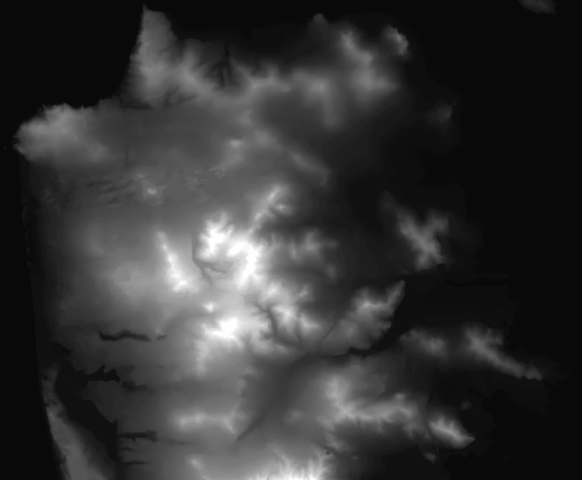
Figure 6-35 shows the elevation contours of San Francisco laid out in a ghostly grayscale, with Twin Peaks and Mt. Sutro standing out as a complex of white in the middle. Now that we have all our data imported into GRASS, we can begin the process of hill shading our topo map in earnest.

Figure 6-35. A composite digital elevation model of San Francisco

 

6.10.4. Applying the Hill Shading

We'll begin this step by using the r.shaded.relief script that comes with GRASS to generate a separate shading layer from our patched DEMs. The r.shaded.relief script uses r.mapcalc internally to calculate the shadows cast by the sun, given its azimuth (or direction) and its height above the horizon. Both the azimuth and the altitude of the sun are measured in degrees. For sake of argument, we'll place the sun due west at 30 degrees high:

GRASS:~/shade > r.shaded.relief azimuth=270 altitude=30 
map=sf_elevation
 
Please provide the altitude of the sun in degrees above the
horizon and the azimuth of the sun in degrees to the east of
north (N:0 E:90 S:180 W:270)
 
Using altitude:30 azimuth:270 elevation:sf_elevation@sderle
 
Running r.mapcalc, please stand by.
Your new map will be named sf_elevation_relshade. Please consider renaming.
 100%
Color table for [sf_elevation_relshade] set to grey
 
Shaded relief map created and named sf_elevation_relshade. Consider renaming.

Our new relief map is stored in a raster layer called sf_elevation_relshade. You can use g.rename to rename it, but we won't bother. If you're curious to know what it looks like, try d.rast sf_elevation_relshade.

In older versions of GRASS, r.shaded.relief was called shade.rel.sh, but the basic details were the same.

Now we want to combine this shading layer with our original topo map to overlay this nifty relief effect. For that, we turn to d.his, which combines hue, intensity, and saturation values (hence his) from two or three raster layers for visual effect. To shade our topo map, we want the hues from the topo map and the intensity from our shading map, which will darken the parts of the topo map that fall into shadow, creating the illusion of relief. The d.his tool is simple to run, and it displays its output immediately, as shown in Figure 6-36:

GRASS:~/shade > d.erase
GRASS:~/shade > d.his h=sf_topo i=sf_elevation_relshade
 100%

Figure 6-36. A shaded relief map of San Francisco

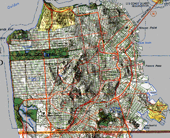
Suddenly, the topographic layout of San Francisco makes sense! You can make out the curved roads that run up and down the sides of the hills and the places where hilltops have been turned into squares or parks. Zooming in reveals the logic of the contour lines in a way that wasn't immediately apparent before. Start another graphics monitor with d.mon start=x1 and use d.rast sf_topo to display the original and the shaded topo maps side by side.

You should play with the azimuth and altitude values provided to r.shaded.relief to get a sense for the hill shading that's most visually appealing to you. Some will definitely look better than others. Read the r.shaded.relief and d.his manpages for more details. Also, you might want to try using the PNG driver to output your map to a graphic that you can share with the world [Hack #75] . Then you should track down the topo maps and elevation data for your own neighborhood and make your own shaded relief maps!

6.10.5. Hacking the Hack

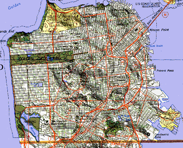
Of course, picking the azimuth and altitude values out of a hat isn't good enough for some people. For the hard-bitten realists among us, there is another option: you can always input the actual height and direction of the sun as it's shining out your window right now (or, at least, where it would be if it were daytime and not sleeting outside, etc.). Although the r.sun and r.sunmask tools provided with GRASS will do some of this math for you, their usage is a little bit complex, and it might be easier to simply get the angle values from another source.

One option is the NOAA Solar Position Calculator at http://www.srrb.noaa.gov/highlights/sunrise/azel.html. You can select your location from a drop-down box of cities, or provide your own latitude and longitude, as well as select the date and time that you want a solar position estimate for. A JavaScript-powered calculator then provides estimates of solar altitude and azimuth, plus a bunch of other figures, for the given place and time. We chose San Francisco at 2:00 pm (GMT -8) on March 18, 2004, approximately the time of this writing, and got values of 219 degrees azimuth and 44 degrees altitude. Figure 6-37 shows the resulting relief map, which, frankly, looks a bit nicer than the one made with the values we invented earlier!

Figure 6-37. A shaded relief map of San Francisco, calculated from actual solar angles