Hack 76. Explore the Effects of Global Warming

See what sea-level change means for the world's coastlines and the people who live near them.

If present trends in greenhouse gas production, deforestation, and average surface temperature continue, it seems likely that Earth's ice caps will continue to melt, dumping untold quantities of water back into the oceans from whence they came and causing sea levels to rise all around the world. Of course, the consequences of such an event would be dramatic, but what exactly would be the result? Where would Earth's new coastlines lie? How many people might be affected? Questions like these can reveal the full power of GIS, which allows us to poseand hopefully answer"what if?" queries that have a geospatial component.

6.14.1. Importing the Elevation Data

The first part of this questionwhere will the new coastlines bedepends on where the current coastlines are. We can start by getting a one-kilometer resolution digital elevation model (DEM) from the GLOBE Project and importing it into GRASS. The GLOBE project's site is http://www.ngdc.noaa.gov/seg/topo/globe.shtml, but you can get the data directly from http://www.ngdc.noaa.gov/seg/topo/globeget.shtml. Click the link to "Select Your Own Area," and you'll be taken to a form where you can specify the details of the DEM you want. Select the Custom... region from the drop-down box on the left and then enter the bounding box for the DEM. We selected -12 degrees for the western edge, 30 degrees for the eastern edge, 65 degrees for the northern edge, and 34 for the southern edge. Beneath the extent selection area, you'll see a whole raft of datafile formatting options. Select ESRI ArcView as your "Export type," a "Data type" of int16, Compressed TAR file as the "Compression option," and FTP as the "Transfer option." Give the data set a custom filename like europe_dem. Finally, click "Get Data." You'll be taken to a download page that will update periodically with the progress of the data set assembly on the server side, which takes about a minute. (Note the cute stick figure juggling 10 balls!) Finally, your browser will download the tarball, which should weigh in at about 13 MB.

The DEM will be in ESRI Binary Interleaved, or BIL format, which can fortuitously be read by GRASS's r.in.gdal tool. Make a new directory, and unpack the tarball inside it:

GRASS 5.7.0:~ > mkdir climate
GRASS 5.7.0:~ > cd climate
GRASS 5.7.0:~/climate > tar xvfz ~/Desktop/europe_dem.tgz
europe_dem.bil
europe_dem.hdr
europe_dem.clr
GRASS 5.7.0:~/climate > r.in.gdal -o in=europe_dem.bil out=dem
 100%
CREATING SUPPORT FILES FOR dem

The tarball contains three files: a .bil file that contains the actual elevation data, a .hdr file that contains the metadata, and a .clr file that contains a default color map. We use r.in.gdal to parse the BIL file into a raster layer called dem. The -o option of r.in.gdal tells it to ignore the fact that the BIL file has no associated projection information. This isn't problematic, as the DEM data is referenced with geographic coordinates (i.e., latitude and longitude) and isn't in a particular projection.

r.in.gdal only recently acquired the ability to automatically load BIL files into the right extents. If your installed version of the GDAL library is older than 1.2.1, you may have to use r.in.bin, which has a significantly more complex syntax. This might be a good excuse to get newer versions of GDAL and GRASS, or maybe trying rebuilding them from source!

We can assign a simple green-yellow-red color map to the dem layer, set the current region to that of the raster layer, and then display it on an X monitor:

GRASS 5.7.0:~/climate > r.colors dem color=gyr
Color table for [dem] set to gyr
GRASS 5.7.0:~/climate > g.region rast=dem
GRASS 5.7.0:~/climate > d.mon start=x0
using default visual which is TrueColor
ncolors: 16777216
Graphics driver [x0] started
GRASS 5.7.0:~/climate > d.rast dem bg=blue
 100%

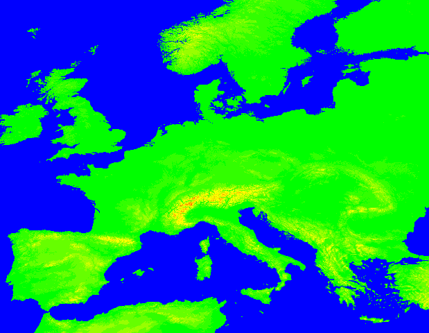
Since the DEM layer import sets existing ocean cell values to null (i.e., no value), we use the bg parameter of d.rast to display these background cells as blue, instead of white. Figure 6-47 shows the result. Now we can start to examine what the coastlines will look like if the sea levels rise.

Figure 6-47. A colorized elevation model of Western Europe

 

6.14.2. Method 1: Hacking the Color Table

Let us suppose the effect of global warming is to cause sea levels to rise by 10 meters, or about 32 feet. This is hopefully a very pessimistic prediction, but it will serve to highlight the effects in question. There are two ways of approaching our visualization of the resulting coastline. The really hackish approach, which we will look at first, is to leave the data itself alone but hack the DEM layer's color table, so that the submerged bits appear to be underwater.

First, let's assign a custom color map to the DEM, using the rules option of r.colors, which lets us specify a set of values (in this case, elevation in meters) and a color to assign to each one. GRASS will then shade each cell in the DEM relative to the values we specify in our color map:

GRASS 5.7.0:~/climate > r.colors dem color=rules
Enter rules, "end" when done, "help" if you need it.
Data range is -103 to 4570
> -103 blue
> 0 green
> 1000 yellow
> 4570 red
> end
Color table for [dem] set to rules
GRASS 5.7.0:~/climate > d.redraw
 100%

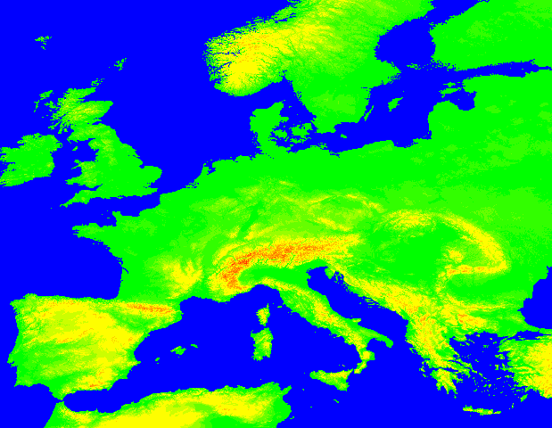
In essence, this color map says, "Color all the cells below sea level in blue shades, land near sea level in green, land from there up to 1000 meters in increasingly yellow shades, land higher than 1000 meters in increasingly red shades up to 4570 meters, our maximum value." Figure 6-48 shows the result, in which the topography of Western Europe stands out a little more strongly than in the previous figure.

Figure 6-48. Western Europe, sporting a custom color map

User-supplied color maps in GRASS don't have to completely cover the range of values in the raster layer, but r.colors will complain if they don't. You can also use r.info to find out what the range is before creating a new color map.

Now, if we want to visualize which parts of Western Europe will be underwater if the sea level rises 10 meters, the easiest way to do so is to just adjust the color map so we see blue all the way up to 10 meters. To make the color map easier to tweak, we can dump the following rules into in a text file called dem.rules:

-103 blue
10 blue
11 green
1000 yellow
4570 red

The new set of color map rules says "Turn everything up to 10 meters blue and make the rest green, yellow, and red as before." We feed dem.rules into r.colors via redirectionthis is a Unix shell, after all! Figure 6-49 shows the result of raising the apparent sea level to 10 meters by hacking the color map:

GRASS 5.7.0:~/climate > r.colors dem color=rules 
Color table for [dem] set to rules
GRASS 5.7.0:~/climate > d.redraw
 100%

Figure 6-49. Western Europe, with apparent sea level raised to 10 meters

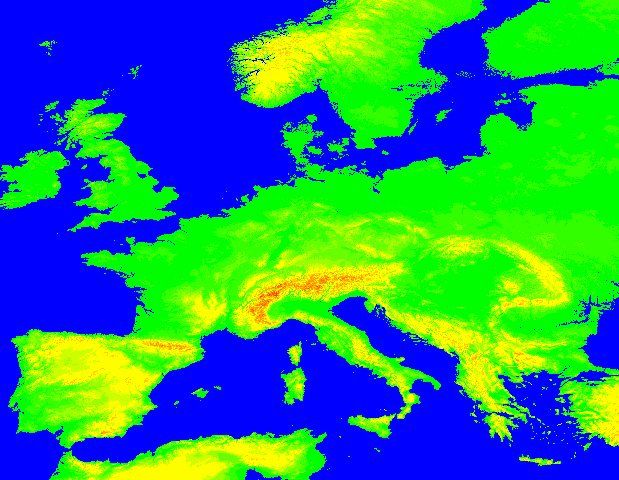
The first thing we notice is that the Netherlands almost disappear completely! Additionally, major cities like London, Copenhagen, and Venice fare rather poorly. This visualization practically begs our other question: if the sea level were to rise by 10 meters, how many people might be displaced? To address this question, we'll have to redo our analysis to specifically identify which cells in our DEM raster will be submerged.

6.14.3. Method 2: Applying Raster Algebra

Our second approach will use raster algebra to identify which parts of our elevation model lie below 10 meters, and hence are at risk of being submerged. Raster algebra is simply any process that derives each cell of a new output layer by applying a user-specified equation to each corresponding cell in a set of input layers. The r.mapcalc tool performs this function in GRASS:

GRASS 5.7.0:~/climate > r.mapcalc 'submerged = if(dem <= 10, 1, null( ))'
 100%
GRASS 5.7.0:~/climate > r.colors submerged color=rules
Enter rules, "end" when done, "help" if you need it.
Data range is 1 to 1
> 1 blue
> end
Color table for [submerged] set to rules

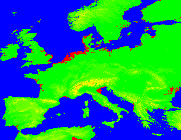
Our call to r.mapcalc creates a new layer called submerged, which contains a value of 1 everywhere dem contains a value less than or equal to 10, and a null value everywhere else. This gives us a raster layer that consists solely of the land areas that would be submerged, which we then color blue. If we reset the colors of our dem layer, we can display the original coastlines subsequently overlaid with the new coastline, giving us a map that looks schematically similar to the map we made in Figure 6-49:

GRASS 5.7.0:~/climate > r.colors dem color=gyr
Color table for [dem] set to gyr
GRASS 5.7.0:~/climate > d.erase
GRASS 5.7.0:~/climate > d.rast dem bg=blue
 100%
GRASS 5.7.0:~/climate > d.rast -o submerged
 100%

The -o option to d.rast causes it to filter out the null values in submerged, rather than erasing the dem layer underneath, resulting in an overlay effect. If we want to highlight, rather than blend in, the submerged areas, we can assign a different color to that layer and redraw. Figure 6-50 shows the highlighted areas overlaid on the original map.

GRASS 5.7.0:~/climate > r.colors submerged color=rules
Enter rules, "end" when done, "help" if you need it.
Data range is 1 to 1
> 1 red
> end
Color table for [submerged] set to rules
GRASS 5.7.0:~/climate > d.redraw
 100%

Figure 6-50. Western Europe, with potentially submerged areas highlighted

All of the potential elaborations of this idea, such as using r.mapcalc to combine the original and submerged land areas into a single layer or using v.in.ascii (or s.in.ascii in GRASS 5.3 and earlier) to import and overlay a map of major European cities, are left as exercises for the reader, so that we can get back to our second question.

You may have noticed a fallacy in our consideration of rising sea levels, which is the assumption that all land areas below our new, hypothetical sea level will be automatically submerged, whether or not the areas are anywhere near an ocean. After all, even in contemporary Europe, significant land areas lie below sea level, sometimes as a result of human intervention. A proper GIS treatment of the subject would take hydrology models, geodetic models, meteorological patterns, and other factors into account, and so our naïve analysis, is at best, a first approximation. We did say it was a hack!

 

6.14.4. Adding Population Data into the Mix

At last, we return to our second question: how many people in Western Europe might be affected by a 10-meter rise in global sea level? To answer this, we will need to import a layer containing population data, which we can combine with our elevation layers to begin making estimates. The "Gridded Population Map of the World," offered by Colombia University's Center for International Earth Information Science Network at http://sedac.ciesin.org/plue/gpw/, is an excellent source of global population data. Download the binary version of their most recent adjusted population data for Europe (from 1995, as of this writing) from ftp://ftp.ciesin.org/pub/gpw/europe/v2eup95agi.zip and unpack it into your working directory. Inside you'll find another BIL data set, which, in principle, should be imported into GRASS in the same fashion as the elevation data we imported earlier:

GRASS 5.7.0:~/climate > unzip v2eup95agi.zip 
Archive: v2eup95agi.zip
 inflating: eup95agi.bil 
 inflating: eup95agi.blw 
 inflating: eup95agi.hdr 
 extracting: eup95agi.stx 
 inflating: readme.txt

However, in practice, the GDAL driver has no way to distinguish between 32-bit floating point values and the 32-bit integers actually stored in the BIL file, due to a bug in the BIL format specification. There are two ways around this. One is to use r.in.bin, but that means calculating the extents of the file by hand. The other way is to use GDAL's "virtual raster" driver to explicitly specify the file structure of the BIL file by means of a separate XML file. We'll take the latter approach. If you run gdalinfo on the data set, you can get the extents and spatial resolution (i.e., degrees per pixel) of the raster layer. We'll use the -mm option to have GDAL count the minimum and maximum values, just to verify that it has trouble with this data set:

GRASS 5.7.0:~/gis/europe > gdalinfo -mm eup95agi.bil
Driver: EHdr/ESRI .hdr Labelled
Size is 1680, 1320
Coordinate System is `'
Origin = (-25.000000,85.000000)
Pixel Size = (0.04166667,-0.04166667)
Corner Coordinates:
Upper Left ( -25.0000000, 85.0000000) 
Lower Left ( -25.0000000, 30.0000000) 
Upper Right ( 45.0000000, 85.0000000) 
Lower Right ( 45.0000000, 30.0000000) 
Center ( 10.0000000, 57.5000000) 
Band 1 Block=1680x1 Type=Float32, ColorInterp=Undefined
 Computed Min/Max=0.000,0.000

As you can see, GDAL gets the minimum and maximum values wrong, as well as the data type (Float32 instead of Int32). Using the geographic origin, and the layer height, width, and pixel size indicated by gdalinfo, we can create a GDAL virtual-raster description that explicitly sets the cell data type to 32-bit integer. Fire up a text editor and dump the following to a file called eup95agi.vrt:

 -25,0.0416666667,0,85,0,-0.0416666667
 
 eup95agi.bil
 MSB
 

As you can see, we've copied in the raster filename, as well as its height and width. The format of the GeoTransform element is (X origin, X resolution, X rotation, Y origin, Y rotation, Y resolution), where the origin is the geographic coordinates of the upper lefthand corner of the layer, as given by GDAL. We copied in the origin and resolution values from gdalinfo and left the rotation values at zero, since we presume that the image is oriented north-up. Finally, we set the byte order to most significant byte first, or MSB (which you can derive yourself by examining the eup95agi.hdr file).

The other option for ByteOrder is least significant byte first, or LSB. The difference is the same as the little-endian/big-endian byte ordering that distinguishes different computing architectures. When dealing with raw GIS data (e.g., BIL format data), your best bet is usually to pick one, and if that gives you really bizarre values, then try the other. In general, bizarre values in GIS data sets are often a sign of data-type or byte-order issues. The GDAL virtual driver, which is documented at http://gdal.org/gdal_vrttut.html, can really come in handy when dealing with these circumstances.

Now you can treat this XML file as if it were an ordinary GDAL layer, by running the following in GRASS:

GRASS 5.7.0:~/climate > r.in.gdal -o in=eup95agi.vrt out=population
 100%
CREATING SUPPORT FILES FOR population

In our new population layer, each cell has a value equal to the estimated number of people that lived in the area represented by that cell in 1995. Unlike the elevation data, the population data doesn't differentiate between water areas and places that are simply uninhabited, which would appear as an undifferentiated mess if you ran d.rast population at this point. (Try it and see, if you like. d.what.rast can be used to query individual raster cells with your mouse.)

To address this, we'll employ r.null to set unpopulated areas in our population data set to "No Value." For good measure, we will replace the original population layer with the new one and assign it a custom color map, since none of the built-in color maps look very good with it:

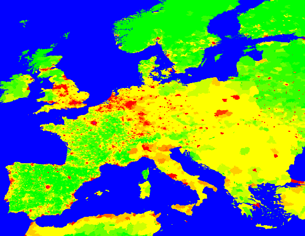
GRASS 5.7.0:~/gis/europe > r.null population setnull=0
Writing new data for [population]... 100%
GRASS 5.7.0:~/climate > r.colors population color=rules
Enter rules, "end" when done, "help" if you need it.
Data range is 0 to 626281
> 0 green
> 1000 yellow
> 10000 red
> 700000 purple
> end
Color table for [population] set to rules
GRASS 5.7.0:~/climate > d.erase
GRASS 5.7.0:~/climate > d.rast population bg=blue
 100%

Once the custom color map is applied, we get a very nice looking population map of Europe, as shown in Figure 6-51.

Figure 6-51. A population map of Western Europe

 

6.14.5. Estimating Population Displacement

Now, back to our second question, which was, "How many people in Western Europe will be displaced from their homes by a 10-meter rise in sea level?" We are finally at the point where we can estimate this number, by tallying up the values of all the cells in our population layer that match the non-null cells in our submerged layer. Fortunately, GRASS provides a function for summing all the values of a given raster layer, and, if you already guessed that this function was called r.sum, give yourself a gold star.

As a check, let's run r.sum on our population layer and see if it produces a reasonable value. In order to make this work, we'll need to make sure that the resolution of the current GRASS region matches that of the population layer, or some values might end up being counted multiple times, which will throw the sum off. Running r.info on the population layer yields the following metadata:

GRASS 5.7.0:~/climate > r.info population
...
 | N: 85N S: 30N Res: 0:02:30 |
 | E: 45E W: 25W Res: 0:02:30 
...

This tells us that the spatial resolution of the image is 2.5 minutes per pixel. We can feed this value directly into g.region and then run r.sum on the population layer:

GRASS 5.7.0:~/gis/europe > g.region res=0:02:30
GRASS 5.7.0:~/gis/europe > r.sum population
Reading pop... 100%
SUM = 604283674.000000

The value we get back, around 604 million, seems about right for the area depicted on our graphics monitor. Now let's create a displaced layer that contains the population values for all the areas in the submerged layer. In order to do this, the submerged layer and the population layer have to have the same resolution, or we'll be comparing apples to oranges. We can use r.resample to down-sample our submerged layer to the resolution of the population layer, and then use r.mapcalc to synthesize the displaced layer:

GRASS 5.7.0:~/gis/europe > r.resample in=submerged out=submerged2
percent complete: 100%
Creating support files for submerged2
creating new cats file...
GRASS 5.7.0:~/gis/europe > r.mapcalc 'displaced = 
if(isnull(submerged), null( ), population)' 100%

Finally, we can use r.sum to estimate how many people live in the potentially submerged areas:

GRASS 5.7.0:~/gis/europe > r.sum displaced
Reading displaced... 100%
SUM = 41109241.000000

Our answer is that about 41 million people will be displaced from their homes in Western and Central Europe, should the current sea levels rise by 10 meters. That's more than one in every 15 people! If we perform the same analysis for the East Coast of the United States, we find that as many as 25 million people there may be displaced, and, mind you, all this is based on population data that is already 10 years old. We haven't performed this analysis for, say, Bangladesh or Southeast Asia, but you can do the math yourself.

6 15 Conclusion