Hack 74. Plot Wireless Network Viewsheds with GRASS

With a little GRASS scripting, you can build sophisticated models of radio-frequency reception for wireless network planningand find out where the black holes are.

If your local terrain is hilly, planning wireless community networks can be a big hassle, as 802.11 depends on line-of-sight between nodes. "Planning" is somewhat of a misnomer; networks grow organically according to movements of people. When you move to a new town, the question "Can I get on your free network?" is most often answered with "We don't know!" Before we start hanging out of the window waving an antenna about, we can start answering this question with viewshed maps, which display the area visible from a given point on an elevation model. Knowing where you can't get directly connected from is a good start.

In [Hack #18], we used a tool called SPLAT! for mapping radio viewsheds. Although SPLAT! is easy to use, it also has several shortcomings. In this hack, we'll look at doing much more sophisticated modeling with GRASS. Using GRASS, we can map wireless viewsheds over any arbitrary base map, taking terrain effects and antenna height, angle, and beam width into account.

Being geeks, when we moved to San Francisco, the first thing we wanted to do was get connected to SFLan, the wireless community network spearheaded by the wonderful Internet Archive. SFLan's home on the Web is at http://archive.org/sflan/. We'll use GRASS to plot a viewshed for SFLan node #11, which is situated on a tower at the peak of San Francisco's Mount Olympus, to a couple of locations in the friendly Potrero Hill and Bernal Heights neighborhoods, and see if we might have line-of-sight to SFLan11.

6.12.1. Loading the Terrain into GRASS

For this hack, we'll use the digital elevation model and digital raster graphic that we imported into GRASS for [Hack #72] . Load GRASS with the San_Francisco location we created in that hack. Then load the stored region we created for San Francisco and call up the USGS digital raster graphic stored in the sf_topo raster layer:

GRASS:~/hacks/viewshed > d.mon start=x0
GRASS:~/hacks/viewshed > g.region san_francisco
GRASS:~/hacks/viewshed > d.rast sf_topo
100%

Next, let's import our three locations into GRASS as a site layer. We'll put the locations into a tab-delimited text file called sites.txt as follows:

-122.4444 37.7631 SFLan11
-122.4008 37.7576 Potrero
-122.4197 37.7394 Bernal

Our three fields are longitude and latitude in the WGS84 datum, and a site label. Of course, longitude comes first, as it's the x-coordinate in our pair, and the longitude values are negative, as they are all west of the prime meridian. Our GRASS location is projected into UTM zone 10 against the NAD27 datum, as we can see from the output of g.proj, excerpted here:

GRASS:~/hacks/viewshed > g.proj -p
-----------------------------------------------------------
PROJ_INFO file:
name: UTM
datum: nad27
dx: -22.000000
dy: 157.000000
dz: 176.000000
proj: utm
ellps: clark66

In earlier versions of GRASS, the g.projinfo tool was the primary means of querying the current GRASS location's projection.

We need to convert our data to UTM and NAD27 before importing it into GRASS, so that the two different projections match up. We can use the proj utility, which isn't part of GRASS, but is a utility from the PROJ.4 cartographic projection library. If you don't have PROJ.4, you can get it from Debian APT with apt-get install proj, or from its homepage at http://www.remotesensing.org/proj/ in a variety of forms. The proj utility accepts coordinates, one pair per line, in a source projection, and outputs the same coordinates in the specified target projection. We'll use proj to convert our sites.txt file from lat/long against WGS84 to UTM zone 10 against NAD27:

GRASS:~/hacks/viewshed > proj +proj=utm +zone=10 +datum=NAD27 sites.txt > sites_utm.txt
GRASS:~/hacks/viewshed > cat sites_utm.txt
548938.11 4179471.21 SFLan11
552782.41 4178884.71 Potrero
551130.05 4176854.99 Bernal

Now we can import sites_utm.txt directly into a vector layer called nodes in GRASS, by feeding the file into the standard input of the v.in.ascii utility. However, v.in.ascii expects the data to be separated by pipe (|) characters, so we'll have to use the standard Unix tr command to change the delimiter for us:

GRASS:~/hacks/viewshed > tr '	' '|' < sites_utm.txt | v.in.ascii out=nodes

Next, we can display these points, and then label them, with the following commands:

GRASS:~/hacks/viewshed > d.vect nodes display=shape 
icon=basic/box color=blue 
GRASS:~/hacks/viewshed > d.vect nodes display=attr attrcol=str_1 
lcolor=blue bgcolor=white xref=left yref=bottom

The display=attr option to d.vect instructs it to display shape attributes, rather than the shapes themselves. In GRASS 5.7, every shape in a vector layer is potentially associated with a row of attributeslabels, statistics, and so onstored in data tables inside GRASS. We don't really have the space to get into why v.in.ascii put the labels into an attribute column with the unimaginative title of str_1, but if you're interested, try running v.info -c nodes, and possibly echo "select * from nodes" | db.select (really!) to see how this sort of thing works under the hood.

In versions prior to GRASS 5.7, point data was stored in separate site layers, rather than as vector layers containing points. If you're running an older version of GRASS, you'll need to use the following commands instead:

GRASS:~/hacks/viewshed > s.in.ascii sites=nodes  in=sites_utm.txt
GRASS:~/hacks/viewshed > d.sites nodes color=blue  type=box
GRASS:~/hacks/viewshed > d.site.labels nodes  color=blue back=white xref=left yref=bottom

Consult the manpages for each of these commands for further details.

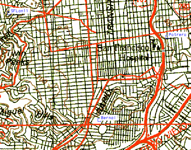
At this point, you should see all three locations appear over the map of San Francisco on the graphics monitor. Now, use the d.zoom tool to constrain our viewing region to an area that just includes our three nodes. We ended up with a region extending from (4176114, 548712) to (4179786, 553358). You can set this region manually in GRASS by typing g.region s=4176114 w=548712 n=4179786 e=553358 and then save the region with g.region save=sflan. You can then recall it at any time with g.region sflan. After doing this, run d.redraw to refresh your display. Figure 6-41 shows the zoomed-in map with all three sites displayed.

Figure 6-41. Map showing potential SFLan sites

 

6.12.2. Making the Radio Viewshed Layer

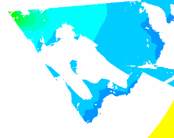
Now that we have our locations set in GRASS, we could go ahead and run the r.los tool, which plots a viewshed from a given location (i.e., the total area to which that location has line of sight) against an elevation layer. However, r.los plots the viewshed in all directions, which we decidedly don't want; the SFLan11 node probably has a directional antenna on its tower, with approximately a 60-degree beam width. Any receiver falling outside that 60-degree arc originating from SFLan11 is going to have a hard time getting a signal, even if it might otherwise have line of sight.

Fortunately, r.los has a patt_map, or pattern map, option, which lets us limit the area to which r.los plots line of sight by supplying a raster layer containing a value of 1 in every cell we want line of sight for, and a 0 in every cell we don't. We're going to have to generate this pattern-map layer from scratch, unfortunately, because GRASS doesn't offer a built-in way of plotting arcs in a given direction from an arbitrary location.

Fortunately, GRASS does offer the extremely powerful and complex r.mapcalc tool, which allows us to feed it equations, perhaps based on values from existing map layers, and output the results of those equations to a new raster layer. Among r.mapcalc's supported functions is the conventional two-argument atan() function. We give it the difference along the x- and y-axes between our origin and our destination, and get back the bearing in degrees between the two points. If the bearing to any arbitrary point falls within the arc direction and beam width, then we include that point in our pattern map; otherwise, we leave it out. (Note that r.mapcalc does loads more than this; take a look at its manpage to get a sense of its scope.)

6.12.3. Generating the Line-of-Sight Layer

The following is the entirety of a GRASS script we concocted called r.slice.sh, a shell script that wraps r.mapcalc to generate r.los pattern-map layers:

#!/bin/bash for i do case $i in arc=*) arc=${i#arc=} ;; azi*=*) azimuth=${i#azi*=} ;; map=*) map=${i#map=} ;; coord*=*) coord=${i#coord*=}; x=${coord%,*}; y=${coord#*,} ;; esac done if [ ! "$arc" -o ! "$azimuth" -o ! "$map" -o ! "$x" -o ! "$y" ]; then echo "Usage: $(basename $0)" echo " map=raster coordinates=x,y arc=value azimuth=value" exit -1 fi r.mapcalc <= min) && (theta <= max)) || \ ((theta - 360 >= min) && (theta - 360 <= max)), \ 1, 0 ) \ ) EOF r.colors map=$map color=rules <

Once we have all the parameters we need, we feed them into r.mapcalc using shell substitution in a here document. The extra clause in the r.mapcalc code involving the theta - 360 calculation handles the edge case where the antenna arc crosses the 0-degree line. Finally, the script assigns a simple black and white color map to our new antenna-arc layer, to make it easy to view.

Now, assuming that SFLan11 has a 60-degree panel pointed to the southeast at 115 degrees true, we can use r.slice.sh to generate our antenna-arc layer like so:

GRASS:~/hacks/viewshed > ./r.slice.sh map=antenna_arc coord=548938.11,4179471.21 azi=115 arc=60
100%
Color table for [antenna_arc] set to rules

 

The coordinates for SFLan11 have simply been taken from sites_utm.txt. Use d.rast antenna_arc to view the resulting raster layer, shown in Figure 6-42.

Figure 6-42. Map showing antenna arc

 

With our new pattern-map layer, we can make realistic models of our wireless viewshed. Feed it to r.los, along with the elevation model loaded from [Hack #72] in the raster layer called sf_elevation. Typically, r.los takes a very long time to runespecially on large regions, where the time to run seems to grow exponentially with the size of the region, which is one of the reasons we zoomed in on our area of interest earlier. Here's the call to r.los:

GRASS:~/hacks/viewshed > r.los in=sf_elevation out=los 
coord=548938.11,4179471.21 patt_map=antenna_arc obs_elev=25 max_dist=5000
 100%

 

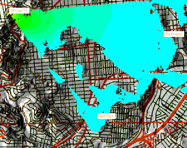
The obs_elev parameter to r.los tells it that the observer (really, the transmitter in this case) is 25 meters above ground level, and the max_dist parameter specifies line-of-sight calculations out to 5 kilometers from the viewing point. The viewshed is written to a raster layer we called los. This command took seven and a half minutes to run on a 1 GHz laptop running Debian Linux! The progress indicator for r.los appears to advance inconsistently, so don't take that as an absolute measure of its actual progress, either. Let's view the new layer in our display using d.rast los, as shown in Figure 6-43.

Figure 6-43. Line-of-sight plot

 

The new line-of-sight layer is colored according to the vertical angle between the transmitter and each point in the viewshed. The yellow arc you see at the bottom right of the layer is where r.los wrote values of zero into the layer because those points were beyond the 5000-meter limit specified by max_dist. Really, those values should be null (i.e., no data) instead of zero, so that they don't interfere with the display of underlying layers when we put everything together, so let's use the r.null tool to reset them:

GRASS:~/hacks/viewshed > r.null los setnull=0
Writing new data for [los]... 100%
GRASS:~/hacks/viewshed > d.redraw
 100%

 

6.12.4. Superimposing Line-of-Sight and Base Map Layers

Now we can put everything together on one map:

GRASS:~/hacks/viewshed > d.erase
GRASS:~/hacks/viewshed > d.rast sf_topo
 100%
GRASS:~/hacks/viewshed > d.rast -o los
 100%
GRASS:~/hacks/viewshed > d.vect nodes display=shape,attr 
attrcol=str_1 icon=basic/box color=orange lcolor=orange bgcolor=white 
xref=left yref=bottom

 

The -o option to d.rast tells it to overlay the los layer on top of the sf_topo layer, rather than overwriting it, leaving the underlying layer present wherever there are null values in the top layer. Note that we changed the site colors to orange from blue, just to make them a little easier to see over the line-of-sight plot. Figure 6-44 shows the result.

Figure 6-44. Shaded line of sight

 

Not bad, eh? In Potrero Hill and Bernal Heights, we should think about buying wireless equipment, but maybe our friends on the eastern side of both hills should wait until someone closer or more advantageously located gets connected before obtaining their own setup.

The underlying elevation model is still a little hard to visualize, though. If you went through all the steps involved in [Hack #72], you should still have a layer called sf_elevation_relshade in your mapset. You can determine this for sure by running g.list type=rast. If so, we can use the method described in that hack to display a topo relief layer as our base map:

GRASS:~/hacks/viewshed > d.his h_map=sf_topo i_map=sf_elevation_relshade
 100%
GRASS:~/hacks/viewshed > d.rast -o los
 100%

 

You can then plot the sites and site labels as before. The result looks something like Figure 6-45.

Figure 6-45. Relief map with site labels

 

In reality, of course, you can use any base map you like. If we want to dump this map to a graphic file, so that we can share the good news with our friends, we can export this set of layers to a PNG file [Hack #75] .

6.12.5. Caveats

Using GRASS to analyze line of sight for wireless networks still comes with a few caveats. First, you may have noticed that we didn't specify a receiver height; that's because r.los doesn't allow us to do so, so we're stuck with a map that shows us line of sight to a receiver at ground level. In this particular case, it won't make much difference, but one can imagine circumstances where it might. Second, r.los is abysmally slow for anything but the shortest distance plots, and even passing it a pattern map doesn't really speed things up much. One alternative that purports to solve these issues is r.cva, a "cumulative viewshed analysis" tool that ships separately from GRASS and must be built against a compiled GRASS source tree. The r.cva tool runs faster and allows you to specify receiver height, but the calling conventions to r.cva are a bit more complicated, so we'll leave its use as an exercise for the reader. You can get the source for r.cva from http://www.ucl.ac.uk/~tcrnmar/GIS/r.cva.html.

Again, we have to emphasize that analysis from elevation models is only the beginning for building wireless networks. Even if the line-of-sight plot says the network is marginal or it only barely can't be done, you might want to try to set up the link anyway; digital elevation models have been known to be erroneous, or at least inaccurate. Further, no terrain model can properly account for ground clutter, such as buildings and trees. In the end, all this sort of analysis can do is help you prioritize your options to help to figure out which ones are more or less likely to workbut, sometimes, that's all you need to get started.

6.12.6. See Also

• [Hack #18]
• [Hack #72]
• [Hack #75]
• [Hack #19]