Oracle Advanced SELECT Options
There are many SQL Select options available in Oracle that are not commonly used or generated by Crystal Reports but that are very useful in certain reporting situations. In this chapter, many of these options will be covered. The HAVING clause allows filtering at the group level. Set operations let you do set manipulations such as unions and intersections. Hierarchical queries, similar to the Crystal Reports hierarchical grouping feature, are also described, and the WITH clause, which enables a simplified use of temporary tables, will be explained. Finally, the very powerful aggregation and analysis functions available will be covered. These functions let you easily do summarizing, ranking, and other analysis, not possible from a simple SELECT statement before Oracle 9i.
HAVING Clause
Crystal Reports allows you to create selection criteria on grouped data. For a simple example, create a report using the Orders table with the Order_Amount totals grouped by Employee_ID. To do this, put Employee_ID and Order_Amount fields on the report. Group by Employee_ID, subtotal Order_Amount by Employee_ID, and suppress the detail section. Check the SQL query that is generated—you can see this query in Figure 4-1.
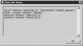
Figure 4-1: SQL for group summary query
Next, specify that you want only those employees whose total Order_Amount exceeds $700,000. Using the Select Expert, create the filter shown in Figure 4-2.
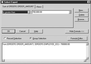
Figure 4-2: Select Expert group selection
Then check the SQL that Crystal generates as shown in Figure 4-3.
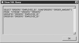
Figure 4-3: SQL for Crystal group selection
You will observe from viewing both screens that the SQL statement has not changed. The number of records returned is 6, one for each Employee_ID. The group filter has not been passed through to Oracle. In the download file, this report is available as Chapter 4Order Amount by Employee with detail hidden with group selection.rpt.
Oracle SQL SELECT statement syntax includes a HAVING clause that is used to filter grouped data. In this case, a query such as the following could be used to do the group filtering on the server:
 SELECT "ORDERS"."EMPLOYEE_ID", SUM("ORDERS"."ORDER_AMOUNT")
 FROM "XTREME"."ORDERS" "ORDERS" GROUP BY "ORDERS"."EMPLOYEE_ID"
 HAVING SUM("ORDERS"."ORDER_AMOUNT")>700000;
You could use this formula in a SQL Command and the filtering would happen on the server with only two records returned, but you would lose the capability to drill down to the detail automatically. However, you could use on-demand subreports to mimic the drill-down capability. In the download file, this is report Chapter 4Order Amount by Employee with on-demand subreport.rpt.
Since automatic drill down and on-demand subreports both issue identical database queries to get the detail data, there is no difference in performance from the database point of view for that portion of the report. However, using the HAVING clause for the main report is optimized for returning only the groups that are needed. The report writer must determine if the trade-off between increased performance and added complexity is worthwhile for any given report.
Set Operations
Using Oracle set operations is not possible if Crystal creates the report query. In order to take advantage of a set operation such as UNION, you must write the query yourself using SQL Commands, stored procedures, views, or Crystal Query files.
UNION
The UNION operation takes the result set of one SELECT statement and appends it to the result set of another SELECT statement. This operation adds rows. Joins, on the other hand, merge rows together so that you get a larger row. UNION creates more rows of the original size.
For example, a phone list is needed that contains the phone numbers for customers, employees, and suppliers in the same report. Phone numbers for each of these entities is stored in a separate corresponding table. A UNION operation allows you to treat them as if they were all in the same table.
SELECT 'Customer' Type,
 Customer_Name Organization,
 Contact_Last_Name Last_Name,
 Contact_First_Name First_Name,
 Phone
 FROM Customer
UNION
SELECT 'Employee', Null,
 Last_Name, First_Name, Home_Phone
 FROM Employee
UNION
SELECT 'Supplier', Supplier_Name,
 Null, Null, Phone
 FROM Supplier
ORDER BY 3, 4
Note that the column names or aliases from the first SELECT statement are the ones used for the entire result set. The number and types of columns in the second and third SELECT statements must match the number and types in the first SELECT statement, though column size can vary. If any duplicate rows are returned, UNION will eliminate them.
An ORDER BY clause is added at the end; this means that the resulting rows from all SELECT statements are sorted as one group. Only one ORDER BY clause is allowed, so individual SELECT statements cannot have their own ORDER BY clause.
UNION ALL
UNION ALL differs from UNION in one respect: UNION ALL will not remove duplicate rows. Because of this, UNION ALL is more efficient than UNION because it does not have to find and eliminate the duplicate rows, but it should be used only if you do not want duplicates eliminated, or if you are certain that there are no duplicates. No sort operation is required.
INTERSECT
INTERSECT returns rows only if they exist in both result sets. For example, the following query would return any phone numbers that show up in any two of the three tables:
 SELECT Phone FROM Customer
 INTERSECT
 SELECT Home_Phone FROM Employee
 UNION
 SELECT Home_Phone FROM Employee
 INTERSECT
 SELECT Phone FROM Supplier
 UNION
 SELECT Phone FROM Customer
 INTERSECT
 SELECT Phone FROM Supplier
Joining this result to the full phone list will return the complete row data for the rows with duplicate phone numbers:
SELECT a.Type, a.Organization, a.Last_Name, a.First_Name,
 Phone
from (SELECT 'Customer' Type,
 Customer_Name Organization,
 Contact_Last_Name Last_Name,
 Contact_First_Name First_Name,
 Phone
 FROM Customer
 UNION ALL
 SELECT 'Employee', Null,
 Last_Name, First_Name, Home_Phone
 FROM Employee
 UNION ALL
 SELECT 'Supplier', Supplier_Name,
 Null, Null, Phone
 FROM Supplier) a
JOIN
 (SELECT Phone FROM Customer
 INTERSECT
 SELECT Home_Phone FROM Employee
 UNION
 SELECT Home_Phone FROM Employee
 INTERSECT
 SELECT Phone FROM Supplier
 UNION
 SELECT Phone FROM Customer
 INTERSECT
 SELECT Phone FROM Supplier) b
USING (Phone)
The preceding query uses the 9i join syntax; the 8i version of this query is located in the download files as Chapter 4Intersect Query for 8i.SQL.
MINUS
The MINUS set operation will return all rows that exist in the first query that do not exist in the second query. It subtracts any rows from the first query that match rows in the second query. Rows that exist in the second query but not the first are not returned.
For example, to find the product_ids for any products that have never been ordered, use the following query.
SELECT product_id FROM product
MINUS
SELECT distinct product_id FROM orders_detail
Hierarchical Queries
Just as Crystal Reports can do hierarchical grouping locally, Oracle can do hierarchical queries on the back end. To create a hierarchical query, you must use the CONNECT BY PRIOR clause. This clause defines the hierarchical relationship similar to the way the WHERE clause defines a join relationship. Though the PRIOR keyword can go on either side of the equality statement, it needs to be associated with the child field. The optional START WITH clause defines the root of the tree. In this case, the SUPERVISOR_ID is null if an employee has no supervisor. The optional ORDER SIBLINGS BY clause is used to sort the rows that are at the same level in the hierarchy:
SELECT employee_id, first_name||' '||last_name Name,
 SYS_CONNECT_BY_PATH(level||' '||First_Name||
 ' '||Last_Name,'') path
FROM employee
START WITH supervisor_id IS NULL
CONNECT BY PRIOR employee_id=supervisor_id
ORDER SIBLINGS BY employee_id
| Note |
The ORDER SIBLINGS BY and SYS_CONNECT_BY_PATH options are new to Oracle 9i. |
The pseudo column Level displays the level of the row in the tree. The rows at the top of the tree are level 1, children of level 1 are level 2, children of level 2 are level 3, and so on. The function SYS_CONNECT_BY_PATH is only valid in a hierarchical query; it is used to create a string containing the path from the top of the tree down to the current row, with a user-defined delimiter separating the levels.
Using Crystal Reports hierarchical grouping features, you can summarize at the tree levels. No such built-in capability exists in Oracle. To duplicate that capability, the SYS_CONNECT_BY_PATH can be parsed to create fields to group by:
SELECT employee_id, Name, salary, position,
 NVL(SUBSTR(path, INSTR(path,'',1,1)+3,
 INSTR(path,'',1,2)-INSTR(path,'',1,1)-3),
 Name) Level_1_Supervisor,
 NVL(SUBSTR(path, INSTR(path,'',1,2)+3,
 INSTR(path,'',1,3)-INSTR(path,'',1,2)-3),
 Name) Level_2_Supervisor
 FROM (SELECT employee_id,
 first_name||' '||last_name Name, salary,
 SYS_CONNECT_BY_PATH(LEVEL||' '||First_Name||'
 '||Last_Name,'') path, position
 FROM employee
 START WITH supervisor_id IS NULL
 CONNECT BY PRIOR employee_id=supervisor_id) p
The Chapter 4Oracle Hierarchy.rpt report shows the result of using the preceding query as a SQL Command for Oracle 9i.
Whether you use Crystal hierarchical grouping or Oracle hierarchical grouping will depend on your needs. Each grouping will result in slightly different displays with their own pros and cons.
WITH Clause
The WITH clause is also known as the subquery factoring clause. The WITH clause precedes the SELECT list and allows you to create temporary tables to use in the SELECT statement. The temporary tables are created in the logged in user’s temporary tablespace automatically. The WITH clause can improve the clarity of statements as well as make them more efficient by storing intermediate results.
| Note |
The subquery factoring clause is new to Oracle 9i. |
The following example computes the minimum modal salary for employees by position:
WITH Counts as
 (SELECT Position, Salary, COUNT(Salary) M
 FROM Employee
 GROUP BY Position, Salary),
 MaxCounts AS
 (SELECT Position, MAX(M) MaxM
 FROM Counts
 GROUP BY Position)
SELECT Counts.Position, MIN(Counts.Salary) Min_Modal_Salary
 FROM Counts, MaxCounts
 WHERE Counts.Position=MaxCounts.Position
 AND Counts.M=MaxCounts.MaxM
 GROUP BY Counts.Position
The preceding example will create two temporary tables, Counts and MaxCounts, from which it will return the final results based on the subsequent SELECT statement.
Aggregation
Oracle 8i and Oracle 9i SQL have some aggregation capabilities that do not exist in standard SQL. These summary operations can be used in SQL Commands, stored procedures, and views.
ROLLUP
ROLLUP and CUBE are extensions to the GROUP BY clause that create additional rows in the result set that contain summary values that would not ordinarily be returned. For instance, the following query containing a ROLLUP command will return records containing the sums at the (country), (country and region), (country, region, and city), and (country, region, city, and customer) grouping levels:
SELECT "CUSTOMER"."COUNTRY", "CUSTOMER"."REGION",
 "CUSTOMER"."CITY", "CUSTOMER"."CUSTOMER_NAME",
 SUM("CUSTOMER"."LAST_YEARS_SALES") SALES,
 DECODE(GROUPING_ID("CUSTOMER"."COUNTRY",
 "CUSTOMER"."REGION",
 "CUSTOMER"."CITY",
 "CUSTOMER"."CUSTOMER_NAME"),
 0,'CUSTOMER',1,'CITY',3,'REGION',
 7,'COUNTRY',15,'GRAND','ERROR') GROUPLEVEL
 FROM "XTREME"."CUSTOMER" "CUSTOMER"
 WHERE ("CUSTOMER"."COUNTRY"='England'
 OR "CUSTOMER"."COUNTRY"='USA')
 GROUP BY ROLLUP ("CUSTOMER"."COUNTRY", "CUSTOMER"."REGION",
 "CUSTOMER"."CITY", "CUSTOMER"."CUSTOMER_NAME")
This query returns the following result:
COUNTRYREGIONCITY CUSTOMER_NAME SALES GROUPLEVEL
------ ----- ------------ --------------------- ---------- --------
USA AL Huntsville Psycho-Cycle 52809.105 CUSTOMER
USA AL Huntsville 52809.105 CITY
USA AL 52809.105 REGION
USA CA Irvine Changing Gears 26705.65 CUSTOMER
USA CA Irvine 26705.65 CITY
USA CA San Diego Sporting Wheels Inc. 85642.56 CUSTOMER
USA CA San Diego 85642.56 CITY
USA CA Newbury Park Rowdy Rims Company 30131.455 CUSTOMER
USA CA Newbury Park 30131.455 CITY
USA CA 142479.665 REGION
USA FL Clearwater Extreme Cycling 69819.1 CUSTOMER
USA FL Clearwater Wheels and Stuff 25556.105 CUSTOMER
USA FL Clearwater 95375.205 CITY
| Note |
The SUPERVISOR_ID function is new to Oracle 9i. |
A query of this type can be used in a Crystal Reports SQL Command to precompute summary values. The rows could be formatted to highlight the summary rows using conditional formatting based on the GROUPING_ID.
The advantage of performing a rollup on the server is minimal in most cases, but it does push all summarization to the server. Even in cases where grouping on the server is taking place in Crystal Reports, only the lowest-level summaries are computed on the server. Higher-level summaries are computed locally. Using ROLLUP, all summaries can be precomputed.
CUBE
The CUBE keyword creates a summary for every possible combination of the GROUP BY fields as in a cross tab. Imagine that you want to know how many employees report to their supervisor. (Crystal’s XTREME data has both a Reports_To and a Supervisor field in its EMPLOYEE table.) The following query will show you where SUPERVISOR_ID is the same as REPORTS_TO, as well as where the fields are not the same, with employee counts for each condition:
SELECT NVL(supervisor_id,0) Supervisor,
 NVL(reports_to,0) Reports_To,
 COUNT(employee_id) NumEmps,
 DECODE(GROUPING_ID(NVL(supervisor_id,0),
 NVL(reports_to,0)),
 0,'Detail',1,'Total for Supervisor_ID',
 2,'Total for Reports_To',
 3,'Grand Total','?') GROUPLEVEL
 FROM employee
 GROUP BY CUBE (NVL(supervisor_id,0), NVL(reports_to,0))
The preceding query returns the following rows:
| Note |
The SUPERVISOR_ID function is new to Oracle 9i. |
SUPERVISOR REPORTS_TO NUMEMPS GROUPLEVEL
---------- ---------- ---------- --------------------------------
 15 Grand Total
 0 2 Total for Reports_To
 2 7 Total for Reports_To
 3 2 Total for Reports_To
 5 3 Total for Reports_To
 13 1 Total for Reports_To
 0 1 Total for Supervisor_ID
 0 0 1 Detail
 2 3 Total for Supervisor_ID
 2 2 3 Detail
 5 7 Total for Supervisor_ID
 5 2 4 Detail
 5 5 3 Detail
 10 2 Total for Supervisor_ID
 10 3 2 Detail
 13 2 Total for Supervisor_ID
 13 0 1 Detail
 13 13 1 Detail
However, the rows returned are not organized in the same way as is generally expected of a cross tab, limiting its usefulness in Crystal Reports.
Analysis
Oracle’s SQL for Analysis is a complex feature. A general overview will be given here, but for a complete description see the Oracle documentation.
The SQL for Analysis functions allow you to do computations that require knowledge of preceding or subsequent rows. Using these functions, you can compute values that would require a stored procedure or complex programming in Crystal Reports.
The analysis functions use the concept of a partition, where a partition is a grouping of rows that the user defines, similar to a GROUP BY in the SELECT statement. Note that this use of the term “partition” is not related to table partitioning and applies only to the statement being processed.
Within a partition, a window may be defined with a starting and an ending point. Either or both the starting point and ending point may move, depending on their definitions. The window may be of any size, from every row in the partition to only one row, and can be based on a number of rows or a time period. If the window is defined to move, it will not move past the partition boundary but will truncate as it approaches the boundary. Therefore, if a moving window from the current row to the next five rows is defined, but the current row is three rows from the end of the partition, only three rows will be included in the computation for the current row. The ending points for a moving window are always defined relative to the current row.
The analysis functions can be broken into several categories covering different capabilities.
Ranking Functions
The ranking functions allow you to compute ranks, percentiles, and other n-tiles. The ranking functions take the following general form:
FUNCTION () OVER ([query_partition_clause] order_by_clause)
The query_partition_clause defines the groups within which the function will be calculated, and the order_by_clause defines the ordering that will be used. The function is reset between partitions. If no partition is defined, the entire result set is assumed. The order_by_clause is similar to a regular ORDER BY for a SELECT statement and has the same defaults. Options for the order_by_clause include ASC/DESC and NULLS FIRST/NULLS LAST. In general, nulls are treated the same as other values and are included in rankings. One null is considered equivalent to another null, and null will be last in an ASC order and first in a DESC order, by default.
RANK
To obtain the ranking of employee_ids by amount ordered, a RANK query such as the following may be used. Note that DESC is used so that the top sellers will be first in the ranking:
SQL> SELECT employee_id, SUM(order_amount) Amount,
 2 Rank () OVER (ORDER BY SUM(order_amount) DESC) Rank
 3 FROM orders
 4 GROUP BY employee_id;


EMPLOYEE_ID AMOUNT RANK
----------- ---------- ----------
 7 748755.94 1
 6 710401.48 2
 9 682849.21 3
 1 660756.95 4
 3 649101.99 5
 4 631799.77 6
To determine the same ranking by order month, modify the query as shown:
SQL> SELECT EXTRACT(MONTH FROM order_date) Month, employee_id,
 2 SUM(order_amount) Amount,
 3 RANK () OVER (PARTITION BY EXTRACT(MONTH FROM order_date)
 4 ORDER BY SUM(order_amount) DESC) Rank
 5 FROM orders
 6 GROUP BY EXTRACT(MONTH FROM order_date), employee_id;


 MONTH EMPLOYEE_ID AMOUNT RANK
---------- ----------- ---------- ----------
 1 6 99979.24 1
 1 9 80512.61 2
 1 7 80182.47 3
 1 1 79581.86 4
 1 4 62453.02 5
 1 3 62129.83 6
 2 9 135328.98 1
 2 6 115022.25 2
 2 3 113115.3 3
 2 7 113057.19 4
 2 4 105110.59 5
 2 1 68762.92 6
More than one ranking function with different partitioning or ordering can be used simultaneously.
Top N rankings can be done as shown to get the top two employees per month:
SQL> SELECT *
 2 FROM (SELECT EXTRACT(MONTH FROM order_date) Month, employee_id,
 3 SUM(order_amount) Amount,
 4 RANK () OVER (PARTITION BY EXTRACT(MONTH FROM order_date)
 5 ORDER BY SUM(order_amount) DESC) Rank
 6 FROM orders
 7 GROUP BY EXTRACT(MONTH FROM order_date), employee_id)
 8 WHERE Rank<3;


 MONTH EMPLOYEE_ID AMOUNT RANK
---------- ----------- ---------- ----------
 1 6 99979.24 1
 1 9 80512.61 2
 2 9 135328.98 1
 2 6 115022.25 2
To get the bottom two employees per month, remove the DESC option:
SQL> SELECT *
 2 FROM (SELECT EXTRACT(MONTH FROM order_date) Month, employee_id,
 3 SUM(order_amount) Amount,
 4 RANK () OVER (PARTITION BY EXTRACT(MONTH FROM order_date)
 5 ORDER BY SUM(order_amount)) Rank
 6 FROM orders
 7 GROUP BY EXTRACT(MONTH FROM order_date), employee_id)
 8 WHERE Rank<3;


 MONTH EMPLOYEE_ID AMOUNT RANK
---------- ----------- ---------- ----------
 1 3 62129.83 1
 1 4 62453.02 2
 2 1 68762.92 1
 2 4 105110.59 2
DENSE_RANK
DENSE_RANK is similar to RANK. Both allow ties, and it is possible that more than one row will have the same rank. The difference between RANK and DENSE_RANK is how the next value after a tie is treated. Imagine that two rows are tied for rank five. When using RANK, the next row’s rank will be seven. When using DENSE_RANK, the next row’s rank will be six.
To demonstrate, the following rounds the order amount to force a tie:
SQL> SELECT employee_id, SUM(order_amount) Amount,
 2 ROUND(SUM(order_amount),-5) Rounded_Amount,
 3 RANK () OVER (ORDER BY SUM(order_amount) DESC) Rank,
 4 RANK () OVER (ORDER BY ROUND(SUM(order_amount),-5) DESC)
 5 Rounded_Rank
 6 FROM orders
 7 GROUP BY employee_id;


EMPLOYEE_ID AMOUNT ROUNDED_AMOUNT RANK ROUNDED_RANK
----------- ---------- -------------- ---------- ------------
 7 748755.94 700000 1 1
 6 710401.48 700000 2 1
 9 682849.21 700000 3 1
 1 660756.95 700000 4 1
 3 649101.99 600000 5 5
 4 631799.77 600000 6 5
Now the Rounded_Rank column has four ties for first place, and the next rank shown is five. Note also that this query shows two different rankings being created simultaneously.
Switching to DENSE_RANK does not affect the Rank columns because it had no ties, but it does affect the Rounded_Rank column, which now shows the next rank as being two rather than five:
SQL> SELECT employee_id, SUM(order_amount) Amount,
 2 ROUND(SUM(order_amount),-5) Rounded_Amount,
 3 DENSE_RANK () OVER (ORDER BY SUM(order_amount) DESC) Rank,
 4 DENSE_RANK () OVER (ORDER BY ROUND(SUM(order_amount),-5) DESC)
 5 Rounded_Rank
 6 FROM orders
 7 GROUP BY employee_id;


EMPLOYEE_ID AMOUNT ROUNDED_AMOUNT RANK ROUNDED_RANK
----------- ---------- -------------- ---------- ------------
 7 748755.94 700000 1 1
 6 710401.48 700000 2 1
 9 682849.21 700000 3 1
 1 660756.95 700000 4 1
 3 649101.99 600000 5 2
 4 631799.77 600000 6 2
CUME_DIST
The cumulative distribution function, CUME_DIST, shows the ratio of the rank of the current row to the rank of the largest row in the set:
SQL> SELECT employee_id, SUM(order_amount) Amount,
 2 RANK () OVER (ORDER BY SUM(order_amount)) Rank,
 3 CUME_DIST () OVER (ORDER BY SUM(order_amount)) Cume_Dist
 4 FROM orders
 5 GROUP BY employee_id;


EMPLOYEE_ID AMOUNT RANK CUME_DIST
----------- ---------- ---------- ----------
 4 631799.77 1 .166666667
 3 649101.99 2 .333333333
 1 660756.95 3 .5
 9 682849.21 4 .666666667
 6 710401.48 5 .833333333
 7 748755.94 6 1
PERCENT_RANK
The PERCENT_RANK function computes the relative position of the rank within the group. It is computed as the current row’s Rank-1 over the group’s largest Rank-1:
SQL> SELECT employee_id, SUM(order_amount) Amount,
 2 RANK () OVER (ORDER BY SUM(order_amount)) Rank,
 3 PERCENT_RANK () OVER (ORDER BY SUM(order_amount)) Percent_Rank
 4 FROM orders
 5 GROUP BY employee_id;


EMPLOYEE_ID AMOUNT RANK PERCENT_RANK
----------- ---------- ---------- ------------
 4 631799.77 1 0
 3 649101.99 2 .2
 1 660756.95 3 .4
 9 682849.21 4 .6
 6 710401.48 5 .8
 7 748755.94 6 1
NTILE
The NTILE function assigns rows to buckets. The following example divides the employees into thirds using their total order amounts:
SQL> SELECT NTILE (3) OVER (ORDER BY SUM(order_amount)) Bucket,
 2 SUM(order_amount) Amount, employee_id
 3 FROM orders
 4 GROUP BY employee_id;


 BUCKET AMOUNT EMPLOYEE_ID
---------- ---------- -----------
 1 631799.77 4
 1 649101.99 3
 2 660756.95 1
 2 682849.21 9
 3 710401.48 6
 3 748755.94 7
Note that the number of rows per bucket can vary if the NTILE number does not divide evenly into the total number of rows. In addition, if the order by expression results in ties, the row could shift buckets depending on the total number of rows, and a tied value could show up in two adjacent buckets.
ROW_NUMBER
The ROW_NUMBER function is similar to RANK, except in its treatment of ties. RANK gives the same value to every row with the same rank, while ROW_NUMBER gives sequential values as shown in the example. The order that the values are assigned within the rank is arbitrary:
SQL> SELECT EXTRACT(MONTH FROM order_date) Month, employee_id,
 2 ROUND(SUM(order_amount),-4) Amount,
 3 RANK () OVER (PARTITION BY EXTRACT(MONTH FROM order_date)
 4 ORDER BY ROUND(SUM(order_amount),-4) DESC) Rank,
 5 ROW_NUMBER () OVER (PARTITION BY EXTRACT(MONTH FROM order_date)
 6 ORDER BY ROUND(SUM(order_amount),-4) DESC) RowN
 7 FROM orders
 8 GROUP BY EXTRACT(MONTH FROM order_date), employee_id;


 MONTH EMPLOYEE_ID AMOUNT RANK ROWNO
---------- ----------- ---------- ---------- ----------
 1 6 100000 1 1
 1 1 80000 2 2
 1 7 80000 2 3
 1 9 80000 2 4
 1 3 60000 5 5
 1 4 60000 5 6
 2 9 140000 1 1
 2 6 120000 2 2
 2 3 110000 3 3
 2 4 110000 3 4
 2 7 110000 3 5
 2 1 70000 6 6
Reporting Aggregate Functions
Reporting aggregate functions are similar to regular SQL aggregates, except that they make the aggregate value available to every detail row and do not cause detail suppression. The reporting aggregates differ from ordinary aggregates such as the simple SUM function. Using a simple SUM returns a sum at the group level of the SELECT statement. Using a reporting aggregate, SUM returns a summary value for every detail row of the SELECT statement at the level defined by the partition clause, independent of the grouping in the SELECT statement.
The syntax for reporting aggregate functions is as follows:
FUNCTION() OVER (partition_by_clause)
The reporting aggregate functions are SUM, AVG, MIN, MAX, COUNT, STDDEV, and VARIANCE. ALL, DISTINCT, and * can be used as they would normally be used with these functions. The partition_by_clause defines the grouping for the aggregation similar to a SQL GROUP BY clause. If no partition_by_clause is given, the aggregate is computed across the entire result set.
Simple Partition Summary
The following example shows a simple sum across a partition. The order amount is summed by employee_id and by month, and the month total is displayed on every row.
SQL> SELECT employee_id, EXTRACT(MONTH FROM order_date) Month,
 2 SUM(order_amount) Amount,
 3 SUM(SUM(order_amount))
 4 OVER (partition by extract(month from order_date)) Month_Total
 5 FROM orders
 6 GROUP BY employee_id, EXTRACT(MONTH FROM order_date);


EMPLOYEE_ID MONTH AMOUNT MONTH_TOTAL
----------- ---------- ---------- -----------
 1 1 79581.86 464839.03
 3 1 62129.83 464839.03
 4 1 62453.02 464839.03
 6 1 99979.24 464839.03
 7 1 80182.47 464839.03
 9 1 80512.61 464839.03
 1 2 68762.92 650397.23
 3 2 113115.3 650397.23
RATIO_TO_REPORT
The RATIO_TO_REPORT function creates ratios of the current record’s value to the partition aggregate value. In the example, you can see that the Percent_of_Total column equals the Amount/Month_Total:
SQL> SELECT employee_id, EXTRACT(MONTH FROM order_date) Month,
 2 SUM(order_amount) Amount,
 3 SUM(sum(order_amount))
 4 OVER (PARTITION BY EXTRACT(MONTH FROM order_date)) Month_Total,
 5 RATIO_TO_REPORT(SUM(order_amount))
 6 OVER (PARTITION BY EXTRACT(MONTH FROM order_date))
 7 Percent_of_Total
 8 FROM orders
 9 GROUP BY employee_id, EXTRACT(MONTH FROM order_date);


EMPLOYEE_ID MONTH AMOUNT MONTH_TOTAL PERCENT_OF_TOTAL
----------- ---------- ---------- ----------- ----------------
 1 1 79581.86 464839.03 .171203051
 3 1 62129.83 464839.03 .133658807
 4 1 62453.02 464839.03 .13435408
 6 1 99979.24 464839.03 .215083574
 7 1 80182.47 464839.03 .172495132
 9 1 80512.61 464839.03 .173205357
 1 2 68762.92 650397.23 .105724497
 3 2 113115.3 650397.23 .173917254
Windowing Aggregate Functions
The windowing functions are an extension of the reporting aggregate functions. They allow you to compute aggregates over a window within a partition. The window is a set of rows where the first row may be fixed or moving and the last row may be fixed or moving, allowing the computation of cumulative aggregates or moving aggregates. The window is always bounded by the partition boundaries.
The windowing aggregate functions are SUM, AVG, MIN, MAX, COUNT, STDDEV, VARIANCE, FIRST_VALUE, and LAST_VALUE. The syntax for a windowing aggregate function is as follows:
FUNCTION(expression) OVER ([query_partition_clause] order_by_clause
 [ROWS or RANGE]
 [[UNBOUNDED PRECEDING or CURRENT ROW
 or expression PRECEDING]
 or
 [BETWEEN [UNBOUNDED PRECEDING or CURRENT ROW
 or expression [PRECEDING or FOLLOWING]]
 AND [UNBOUNDED FOLLOWING or CURRENT ROW
 or expression [PRECEDING or FOLLOWING]]]])
The order_by_clause is not required and not important when using reporting aggregate functions because the summary is computed for the entire group so the order of the rows within the group is irrelevant. When using the windowing aggregate functions, however, the order_by_clause is important because the window will slide across the partition and produce different values if the rows are in a different order.
Cumulative Summary
To display a cumulative aggregation for a partition, you must specify the ROWS UNBOUNDED PRECEDING clause. This will result in all rows from the beginning of the partition up to the current row being aggregated. The following example shows the cumulative order amount, which is identical to a running total in Crystal:
SQL> SELECT employee_id, EXTRACT(MONTH FROM order_date) Month,
 2 SUM(order_amount) Amount,
 3 SUM(SUM(order_amount))
 4 OVER (PARTITION BY EXTRACT(MONTH FROM order_date)
 5 ORDER BY employee_id
 6 ROWS UNBOUNDED PRECEDING) Cum_Month_Total
 7 FROM orders
 8 GROUP BY employee_id, EXTRACT(MONTH FROM order_date);


EMPLOYEE_ID MONTH AMOUNT CUM_MONTH_TOTAL
----------- ---------- ---------- ---------------
 1 1 79581.86 79581.86
 3 1 62129.83 141711.69
 4 1 62453.02 204164.71
 6 1 99979.24 304143.95
 7 1 80182.47 384326.42
 9 1 80512.61 464839.03
 1 2 68762.92 68762.92
 3 2 113115.3 181878.22
If a descending directive is added to the order_by_clause, a different cumulative total will result, illustrating the importance of sort order:
SQL> SELECT employee_id, EXTRACT(MONTH FROM order_date) Month,
 2 SUM(order_amount) Amount,
 3 SUM(SUM(order_amount))
 4 OVER (PARTITION BY EXTRACT(MONTH FROM order_date)
 5 ORDER BY employee_id DESC
 6 ROWS UNBOUNDED PRECEDING) Cum_Month_Total
 7 FROM orders
 8 GROUP BY employee_id, EXTRACT(MONTH FROM order_date);


EMPLOYEE_ID MONTH AMOUNT CUM_MONTH_TOTAL
----------- ---------- ---------- ---------------
 9 1 80512.61 80512.61
 7 1 80182.47 160695.08
 6 1 99979.24 260674.32
 4 1 62453.02 323127.34
 3 1 62129.83 385257.17
 1 1 79581.86 464839.03
 9 2 135328.98 135328.98
 7 2 113057.19 248386.17
Modifying the previous query to partition by employee_id and order_by_month will result in the following SQL, which shows the cumulative order total by employee_id across the months:
SQL> SELECT employee_id, EXTRACT(MONTH FROM order_date) Month,
 2 SUM(order_amount) Amount,
 3 SUM(SUM(order_amount))
 4 OVER (PARTITION BY employee_id
 5 ORDER BY EXTRACT(MONTH FROM order_date)
 6 ROWS UNBOUNDED PRECEDING) Cum_Month_Total
 7 FROM orders
 8 GROUP BY employee_id, EXTRACT(MONTH FROM order_date);


EMPLOYEE_ID MONTH AMOUNT CUM_MONTH_TOTAL
----------- ---------- ---------- ---------------
 1 1 79581.86 79581.86
 1 2 68762.92 148344.78
 1 3 58676.28 207021.06
 1 4 72431.48 279452.54
 1 5 31344.59 310797.13
 1 6 84149 394946.13
 1 7 17991.33 412937.46
 1 8 59291.32 472228.78
 1 9 24894.67 497123.45
 1 10 27652.89 524776.34
 1 11 35127.71 559904.05
 1 12 100852.9 660756.95
 3 1 62129.83 62129.83
 3 2 113115.3 175245.13
Now say that your boss wishes to see how the employee’s monthly average changes through the year:
SQL> SELECT employee_id, EXTRACT(MONTH FROM order_date) Month,
 2 SUM(order_amount) Amount,
 3 AVG(SUM(order_amount))
 4 OVER (PARTITION BY employee_id
 5 ORDER BY EXTRACT(MONTH FROM order_date)
 6 ROWS UNBOUNDED PRECEDING) Running_Average
 7 FROM orders
 8 GROUP BY employee_id, EXTRACT(MONTH FROM order_date);


EMPLOYEE_ID MONTH AMOUNT RUNNING_AVERAGE
----------- ---------- ---------- ---------------
 1 1 79581.86 79581.86
 1 2 68762.92 74172.39
 1 3 58676.28 69007.02
 1 4 72431.48 69863.135
 1 5 31344.59 62159.426
 1 6 84149 65824.355
 1 7 17991.33 58991.0657
 1 8 59291.32 59028.5975
 1 9 24894.67 55235.9389
 1 10 27652.89 52477.634
 1 11 35127.71 50900.3682
 1 12 100852.9 55063.0792
 3 1 62129.83 62129.83
 3 2 113115.3 87622.565
Moving Summary
Then the boss says that only the most recent three months matter. Now you need a moving average over the last three months only. All you need to do is change the UNBOUNDED keyword to two (not three, because the current row is always included):
SQL> SELECT employee_id, EXTRACT(MONTH FROM order_date) Month,
 2 SUM(order_amount) Amount,
 3 AVG(SUM(order_amount))
 4 OVER (PARTITION BY employee_id
 5 ORDER BY EXTRACT(MONTH FROM order_date)
 6 ROWS 2 PRECEDING) Three_Month_Average
 7 FROM orders
 8 GROUP BY employee_id, EXTRACT(MONTH FROM order_date);


EMPLOYEE_ID MONTH AMOUNT THREE_MONTH_AVERAGE
----------- ---------- ---------- ---------------
 1 1 79581.86 79581.86
 1 2 68762.92 74172.39
 1 3 58676.28 69007.02
 1 4 72431.48 66623.56
 1 5 31344.59 54150.7833
 1 6 84149 62641.69
 1 7 17991.33 44494.9733
 1 8 59291.32 53810.55
 1 9 24894.67 34059.1067
 1 10 27652.89 37279.6267
 1 11 35127.71 29225.09
 1 12 100852.9 54544.5
 3 1 62129.83 62129.83
 3 2 113115.3 87622.565
Centered Moving Summary
In retrospect, the boss would also like to see the three-month moving average calculated using the current month, previous month, and the next month. Of course, you must be careful with such computations because presumably next month’s value is only known when the current row is in the past.
SQL> SELECT employee_id, EXTRACT(MONTH FROM order_date) Month,
 2 SUM(order_amount) Amount,
 3 AVG(SUM(order_amount))
 4 OVER (PARTITION BY employee_id
 5 ORDER BY EXTRACT(MONTH FROM order_date)
 6 ROWS BETWEEN 1 PRECEDING AND 1 FOLLOWING)
 7 Three_Month_Centered
 8 FROM orders
 9 GROUP BY employee_id, EXTRACT(MONTH FROM order_date);


EMPLOYEE_ID MONTH AMOUNT THREE_MONTH_CENTERED
----------- ---------- ---------- --------------------
 1 1 79581.86 74172.39
 1 2 68762.92 69007.02
 1 3 58676.28 66623.56
 1 4 72431.48 54150.7833
 1 5 31344.59 62641.69
 1 6 84149 44494.9733
 1 7 17991.33 53810.55
 1 8 59291.32 34059.1067
 1 9 24894.67 37279.6267
 1 10 27652.89 29225.09
 1 11 35127.71 54544.5
 1 12 100852.9 67990.305
 3 1 62129.83 87622.565
 3 2 113115.3 72252.99
Using RANGE
The keyword RANGE can be used with date windows. Windows created with RANGE may have a varying number of rows in them but will have a fixed number of dates. The example query shows a three-day average where the number of detail records per date varies:
SQL> SELECT order_date, order_amount Amount,
 2 SUM(order_amount)
 3 OVER (ORDER BY order_date
 4 RANGE BETWEEN INTERVAL '2' DAY PRECEDING
 5 AND CURRENT ROW) Three_Day_Avg
 6 FROM orders
 7 WHERE order_date BETWEEN TO_DATE('04-01-2002','mm-dd-yyyy')
 8 AND TO_DATE('04-30-2002','mm-dd-yyyy')
 9 ORDER BY order_date;


ORDER_DAT AMOUNT THREE_DAY_AVG
--------- ---------- ---------------
01-APR-02 13.5 57
01-APR-02 43.5 57
02-APR-02 29 86
03-APR-02 55.8 7812.36
03-APR-02 43.5 7812.36
03-APR-02 7534.06 7812.36
03-APR-02 43.5 7812.36
03-APR-02 49.5 7812.36
04-APR-02 9649.2 17404.56
05-APR-02 49.5 17425.06
06-APR-02 1028.55 10854.16
06-APR-02 15.5 10854.16
06-APR-02 45.68 10854.16
06-APR-02 33 10854.16
06-APR-02 32.73 10854.16
Note that a day interval is assumed when the window is based on a date, so the following query has the same result:
SELECT order_date, order_amount Amount,
 SUM(order_amount)
 OVER (ORDER BY order_date
 RANGE BETWEEN 2 PRECEDING AND CURRENT ROW) Three_Day_Avg
 FROM orders
 WHERE order_date BETWEEN TO_DATE('04-01-2002','mm-dd-yyyy')
 AND TO_DATE('04-30-2002','mm-dd-yyyy')
 ORDER BY order_date;
Using an Expression for Number of Rows
An expression can be used for the number of rows in either the PRECEDING or FOLLOWING clauses. A contrived example is shown where the number of days is two if the month is April and three otherwise. A common use for this feature might be to skip holidays by using a function to return the desired number of days.
SQL> SELECT order_date, order_amount Amount,
 2 SUM(order_amount)
 3 OVER (ORDER BY order_date
 4 RANGE BETWEEN DECODE(EXTRACT(MONTH FROM order_date),4,2,3)
 5 PRECEDING AND CURRENT ROW) Day_Avg
 6 FROM orders
 7 WHERE order_date BETWEEN TO_DATE('04-01-2002','mm-dd-yyyy')
 8 AND TO_DATE('04-30-2002','mm-dd-yyyy')
 9 ORDER BY order_date;


ORDER_DAT AMOUNT DAY_AVG
--------- ---------- ----------
01-APR-02 13.5 57
01-APR-02 43.5 57
02-APR-02 29 86
03-APR-02 55.8 7812.36
03-APR-02 43.5 7812.36
03-APR-02 7534.06 7812.36
03-APR-02 43.5 7812.36
03-APR-02 49.5 7812.36
04-APR-02 9649.2 17404.56
05-APR-02 49.5 17425.06
06-APR-02 1028.55 10854.16
06-APR-02 15.5 10854.16
06-APR-02 45.68 10854.16
06-APR-02 33 10854.16
06-APR-02 32.73 10854.16
FIRST_VALUE and LAST_VALUE
The FIRST_VALUE and LAST_VALUE functions return the first or last value in a window, respectively. The example computes the percentage that each employee’s orders were of the largest employee’s orders. Note that this result could have been obtained using the RATIO_TO_REPORT function as well.
SQL> SELECT employee_id, EXTRACT(MONTH FROM order_date) Month,
 2 SUM(order_amount) Amount,
 3 FIRST_VALUE(SUM(order_amount))
 4 OVER (PARTITION BY EXTRACT(MONTH FROM order_date)
 5 ORDER BY SUM(order_amount) DESC) Last,
 6 100*SUM(order_amount)/
 7 FIRST_VALUE(SUM(order_amount))
 8 OVER (PARTITION BY EXTRACT(MONTH FROM order_date)
 9 ORDER BY SUM(order_amount) DESC) Percent_of_Last
 10 FROM orders
 11 GROUP BY employee_id, EXTRACT(MONTH FROM order_date);


EMPLOYEE_ID MONTH AMOUNT LAST PERCENT_OF_LAST
----------- ---------- ---------- ---------- ---------------
 6 1 99979.24 99979.24 100
 9 1 80512.61 99979.24 80.5293279
 7 1 80182.47 99979.24 80.1991193
 1 1 79581.86 99979.24 79.5983846
 4 1 62453.02 99979.24 62.4659879
 3 1 62129.83 99979.24 62.1427308
 9 2 135328.98 135328.98 100
 6 2 115022.25 135328.98 84.9945444
LAG LEAD
The LAG and LEAD functions allow you to reference a value in a row that is a number of rows above or below the current row. The syntax for LAG and LEAD is as follows:
LAG|LEAD (expression [, offset] [, default])
 OVER ([query_partition_clause] order_by_clause)
LAG references rows before the current row, and LEAD references rows after the current row. Null will be returned if the reference row is outside of the partition. The expression is the column or computation to be returned, and the offset is the number of rows to reference forward or back. The offset must be a value and defaults to one. A default can be used to return a user-defined value instead of null when the reference is outside of the partition. The query_partition_clause is optional; if none is supplied, the entire result set will be assumed. The order_by_clause is required.
SQL> SELECT employee_id, EXTRACT(MONTH FROM order_date) Month,
 2 SUM(order_amount) Amount,
 3 LAG(SUM(order_amount),2)
 4 OVER (PARTITION BY EXTRACT(MONTH FROM order_date)
 5 ORDER BY SUM(order_amount) DESC) LAG_2,
 6 LEAD(SUM(order_amount),1,0)
 7 OVER (PARTITION BY EXTRACT(MONTH FROM order_date)
 8 ORDER BY SUM(order_amount) DESC) LEAD_1
 9 FROM orders
 10 GROUP BY employee_id, EXTRACT(MONTH FROM order_date);


EMPLOYEE_ID MONTH AMOUNT LAG_2 LEAD_1
----------- ---------- ---------- ---------- ----------
 6 1 99979.24 80512.61
 9 1 80512.61 80182.47
 7 1 80182.47 99979.24 79581.86
 1 1 79581.86 80512.61 62453.02
 4 1 62453.02 80182.47 62129.83
 3 1 62129.83 79581.86 0
 9 2 135328.98 115022.25
 6 2 115022.25 113115.3
FIRST LAST
| Note |
The FIRST and LAST functions are new in Oracle 9i. |
The FIRST and LAST functions allow you to return any column value or any expression computed from the row that is the first or last row returned, given a specified order. This differs from the FIRST_VALUE and LAST_VALUE functions that return the first or last column or expression defined, given the sort order. For example, say that you need the salary, employee_id, and supervisor_id of the employee with the lowest salary. Without the FIRST or LAST function, this would require a subquery as shown:
SQL> SELECT salary Lowest_Salary, employee_id Employee,
 2 supervisor_id Supervisor
 3 FROM employee
 4 WHERE salary=(SELECT MIN(salary) FROM employee);


LOWEST_SALARY EMPLOYEE SUPERVISOR
------------- ---------- ----------
 18000 11 10
The equivalent result can be obtained using the FIRST function as shown.
SQL> Select MIN(salary)
 2 KEEP (DENSE_RANK FIRST ORDER BY salary) Lowest_Salary,
 3 MIN(employee_id)
 4 KEEP (DENSE_RANK FIRST ORDER BY salary) Employee,
 5 MIN(supervisor_id)
 6 KEEP (DENSE_RANK FIRST ORDER BY salary) Supervisor
 7 FROM employee;


LOWEST_SALARY EMPLOYEE SUPERVISOR
------------- ---------- ----------
 18000 11 10
However, what if there were two employees with a salary of $18,000? The first query using a subquery would return both records. The second query that uses the FIRST function would return only one row, but it might contain a mixture of data from each of the employee’s rows. This is probably not desirable but can be cured in either situation by the creation of a tiebreaker condition.
Suppose there is more than one employee with the lowest salary and the employee with the earliest hire_date is desired. There are multiple methods to solve this without using the FIRST function. The example shows a solution using the subquery factoring clause (WITH):
SQL> WITH Poor_Emps AS
 2 (SELECT salary Lowest_Salary, employee_id Employee,
 3 supervisor_id Supervisor, hire_date
 4 FROM employee
 5 WHERE salary=(SELECT MIN(salary) FROM employee))
 6 SELECT Lowest_Salary, Employee, Supervisor
 7 FROM Poor_Emps
 8 WHERE hire_date=(SELECT MIN(hire_date) FROM Poor_Emps);


LOWEST_SALARY EMPLOYEE SUPERVISOR
------------- ---------- ----------
 18000 11 10
Using the FIRST function, the solution requires only adding the tiebreaker field to the sort:
SQL> SELECT MIN(salary)
 2 KEEP (DENSE_RANK FIRST ORDER BY salary,
 3 hire_date) Lowest_Salary,
 4 MIN(employee_id)
 5 KEEP (DENSE_RANK FIRST ORDER BY salary,
 6 hire_date) Employee,
 7 MIN(supervisor_id)
 8 KEEP (DENSE_RANK FIRST ORDER BY salary,
 9 hire_date) Supervisor
 10 FROM employee;


LOWEST_SALARY EMPLOYEE SUPERVISOR
------------- ---------- ----------
 18000 11 10
The FIRST and LAST functions can be used with a partition similar to previous functions that have been covered.
Linear Regression
The linear regression category of functions covers the linear regression statistics that are available. I will show a simple example, but it is beyond the scope of this book to define or discuss in detail the uses of these statistics. Further detail should be sought from Oracle documentation.
Each regression function takes two parameters that can be thought of as (y, x) coordinate pairs, where x is the independent variable and y is the dependent variable.
| Note |
Oracle documentation uses (y, x) NOT (x, y), so that is replicated here. |
REGR_COUNT
REGR_COUNT returns the number of non-null pairs.
REGR_AVGX
REGR_AVGX returns the average of the x values.
REGR_AVGY
REGR_AVGY returns the average of the y values.
REGR_SLOPE
REGR_SLOPE returns the slope of the computed regression line.
REGR_INTERCEPT
REGR_INTERCEPT returns the y intercept of the computed regression line.
REGR_R2
REGR_R2 returns the R-squared or coefficient of determination of the computed regression line.
Other
There are other regression functions, and other measures can be obtained from combinations of functions.
Regression Example
Assume that you are interested in the relationship between salary and length of employment. The example computes several regression statistics, including the REGR_R2, which is not close to one, indicating a weak correlation between salary and length of employment:
SQL> SELECT REGR_SLOPE(Salary, SYSDATE-hire_date) slope,
 2 REGR_INTERCEPT(Salary, SYSDATE-hire_date) Intercept,
 3 REGR_R2(Salary, SYSDATE-hire_date) R_Squared,
 4 REGR_COUNT(Salary, SYSDATE-hire_date) Count,
 5 REGR_AVGX(Salary, SYSDATE-hire_date) Avg_Days,
 6 REGR_AVGY(Salary, SYSDATE-hire_date) Avg_Salary
 7 FROM employee;


 SLOPE INTERCEPT R_SQUARED COUNT AVG_DAYS AVG_SALARY
---------- ---------- ---------- ---------- ---------- ----------
 .74882077 41682.4804 .000198374 15 3807.12317 44533.3333
However, if you group by position to produce the individual statistics for each position, you see that the correlation improves for Sales Representatives, although it does not exist for the other positions because they each have only one data point.
SQL> SELECT position,
 2 REGR_SLOPE(Salary, SYSDATE-hire_date) slope,
 3 REGR_INTERCEPT(Salary, SYSDATE-hire_date) Intercept,
 4 REGR_R2(Salary, SYSDATE-hire_date) R_2,
 5 REGR_COUNT(Salary, SYSDATE-hire_date) Count,
 6 REGR_AVGX(Salary, SYSDATE-hire_date) Avg_Days,
 7 REGR_AVGY(Salary, SYSDATE-hire_date) Avg_Salary
 8 FROM employee
 9 GROUP BY position;


POSITION SLOPE INTERCEPT R_2 COUNT AVG_DAYS AVG_SALARY
---------------------- ----- –-------- ------ ----- -------- ----------
Advertising Specialist 1 3363 45000
Business Manager 1 3700 60000
Inside Sales Coordinator 1 3730 45000
Mail Clerk 1 3745 18000
Marketing Associate 1 3380 50000
Marketing Director 1 3394 75000
Receptionist 1 3625 25000
Sales Manager 1 3869 50000
Sales Representative 2.02 26919.23 .05 6 4001 35000
Vice President, Sales 1 4298 90000
The regression functions can be used as report aggregates, windowing aggregates, or as shown, regular SQL aggregates.
Inverse Percentile
The inverse percentile functions will return the value that corresponds to a particular percentile. This is the opposite of the NTILE functions that return the percentile for a value.
| Note |
The inverse percentile functions are new in Oracle 9i. |
Say that you want to know the median salary. From the following query, you can see that there are 15 salaries, so the median, or middle salary, is the eighth value, or 40,000.
SQL> SELECT ROW_NUMBER() OVER (ORDER BY salary) RowNo, salary
 2 FROM employee
 3 ORDER BY salary;


 ROWNO SALARY
---------- ----------
 1 18000
 2 25000
 3 30000
 4 33000
 5 35000
 6 35000
 7 37000
 8 40000
 9 45000
 10 45000
 11 50000
 12 50000
 13 60000
 14 75000
 15 90000
The median is the value at the .5 percentile, so you can use the inverse percentile functions to obtain it.
SQL> SELECT PERCENTILE_CONT(0.5)
 2 WITHIN GROUP (ORDER BY salary) Median_Continuous,
 3 PERCENTILE_DISC(0.5)
 4 WITHIN GROUP (ORDER BY salary) Median_Discontinuous
 5 FROM employee
 6 ORDER BY salary;


MEDIAN_CONTINUOUS MEDIAN_DISCONTINUOUS
----------–----–- ------------------–-
 40000 40000
The PERCENTILE_CONT function will use linear interpolation between the two middle values if the number of values in the set is even. The PERCENTILE_DISC function will pick the lower value.
If you exclude employee_id 1, you will have the following values in an even numbered set:
SQL> SELECT ROW_NUMBER() OVER (ORDER BY salary) RowNo, salary
 2 FROM employee
 3 WHERE employee_id<> 1
 4 ORDER BY salary;


 ROWNO SALARY
---------- ----------
 1 18000
 2 25000
 3 30000
 4 33000
 5 35000
 6 35000
 7 37000
 8 45000
 9 45000
 10 50000
 11 50000
 12 60000
 13 75000
 14 90000
The continuous median of this set will be between 37,000 and 45,000, and the discontinuous median will be 37,000.
SQL> SELECT PERCENTILE_CONT(0.5)
 2 WITHIN GROUP (ORDER BY salary) Median_Continuous,
 3 PERCENTILE_DISC(0.5)
 4 WITHIN GROUP (ORDER BY salary) Median_Discontinuous
 5 FROM employee
 6 WHERE employee_id<>1
 7 ORDER BY salary;


MEDIAN_CONTINUOUS MEDIAN_DISCONTINUOUS
----------------- --------------------
 41000 37000
The inverse percentile functions can be used for any value, not just the median, and they can be used as regular aggregates or reporting or windowing aggregates. See Oracle documentation for more information.
Hypothetical Rank and Distribution
The hypothetical rank function will return the rank that a row would have if it were inserted into a particular group. RANK, DENSE_RANK, PERCENT_RANK, and CUME_DIST can be used to return the corresponding hypothetical value for a supplied value.
| Note |
The hypothetical rank and distribution functions are new in Oracle 9i. |
Look back at the ranked salary listing in the previous examples. Suppose that you want to know what rank a salary of 36,000 would have if it were inserted into the group. From observation, you can see that it would rank at seventh place, which the query confirms:
SQL> SELECT RANK(36000) WITHIN GROUP (ORDER BY salary) Test_Rank
 2 FROM employee;


 TEST_RANK
----------
 7
The hypothetical rank and distribution functions cannot be used as reporting or windowing functions, only as regular SQL aggregates. See Oracle documentation for more information.
WIDTH_BUCKET
The WIDTH_BUCKET function assigns a bucket number to a value. The user supplies the starting value, ending value, and number of buckets desired. Any values that fall below the starting value are assigned bucket number 0. Any values that are above the ending value are assigned to a bucket numbered one larger than the requested number of buckets.
| Note |
The WIDTH_BUCKET function is new in Oracle 9i. |
Suppose that you want to create a histogram of salaries in $10,000 increments. The following query will assign salaries between $10,000 and $20,000 to bucket 1, salaries between $20,000 and $30,000 to bucket 2, and so on:
SQL> SELECT employee_id, salary,
 2 WIDTH_BUCKET(salary, 10000, 100000, 9) Bucket
 3 FROM employee
 4 ORDER BY 3,2,1;


EMPLOYEE_ID SALARY BUCKET
----------- ---------- ----------
 11 18000 1
 12 25000 2
 6 30000 3
 3 33000 3
 4 35000 3
 9 35000 3
 7 37000 3
 1 40000 4
 8 45000 4
 15 45000 4
 5 50000 5
 14 50000 5
 10 60000 6
 13 75000 7
 2 90000 9
If you need to perform statistical analysis in your reports, refer to more detailed documentation that specifically discusses the practical application of the useful, though often complex, statistical functions available with Oracle 9i.
This chapter covered many obscure and advanced SELECT statement options that can help solve complex reporting needs. In order to implement any of these options using Crystal Reports, the developer must use SQL Commands, views, stored procedures, or Crystal Query files. Though the options listed in this chapter are powerful, some problems require the use of stored procedures. The next chapter will describe the use of Oracle stored procedures in Crystal Reports.
EAN: N/A
Pages: 101
