A Hybrid Clustering Technique to Improve Patient Data Quality

Overview

Narasimhaiah Gorla
Wayne State University, USA

Chow Y. K. Bennon
Hong Kong Polytechnic University, Hong Kong

Copyright © 2003, Idea Group Inc. Copying or distributing in print or electronic forms without written permission of Idea Group Inc. is prohibited.

Abstract

The demographic and clinical description of each patient is recorded in the databases of various hospital information systems. The errors in patient data are: wrong data entry, absence of information provided by the patient, improper identity of the patients (in case of tourists in Hong Kong), etc. These data errors will lead to a phenomenon that records of the same patient will be shown as records of different patients. In order to solve this problem, we use "clustering," a data mining technique, to group "similar" patients together. We used three algorithms: hierarchical clustering, partitioned clustering, and hybrid algorithm combining these two, and applied on the patient data using a C program. We used six attributes of patient data: Sex, DOB, Name, Marital status, District, and Telephone number as the basis for computing similarity, with some weights to the attributes. We found that the Hybrid algorithm gave more accurate grouping compared to the other algorithms, had smaller mean square error, and executed faster. Due to the privacy ordinance, the true data of patients is not shown, but only simulated data is used.

Introduction

The establishment of the Hospital Authority marked the milestone for all public hospitals in Hong Kong. Under the management of the Hospital Authority, the daily operations of the public hospitals are linked and are under the centralized control of Hospital Authority Head Office (HAHO). Whenever a person uses any service of any one of the public hospitals, his/her personal information will be entered into a corresponding clinical information system. All the clinical information systems are linked and share a master database system that is known as the Patient Master Index (PMI). The main function of PMI is to maintain and control the demographic data of patients. Each patient record is identified by his/her Hong Kong Identification Card (HKID) number or Birth Certificate number. The personal data in PMI can be accessed by any linked clinical information system. Whenever the detail of a patient is updated by any linked clinical information system, PMI is updated automatically. Ideally, each patient should have a unique master record in PMI. However, a patient may contain two or more records in the PMI due to reasons, such as: a patient comes to a hospital without his/her HKID, the information of the patient is wrongly reported by a second party; a patient cannot be identified by any valid document, the patient is a non-Hong Kong resident, such as tourist, a baby is born without a Birth Certificate, data entry operators make typing errors.

If any of the above cases occur, a unique pseudo-identification number will be generated by the clinical information system to identify the patient temporarily. Once the HKID or Birth Certificate number is provided by the patient during hospitalization, the personal information will be updated and the pseudo-identification number will be discarded. However, many patients cannot provide their identification documents before they leave the hospital. More temporary records may be generated for the same patient when a patient attends a hospital several times, thus more and more "duplicate" records will be generated in the PMI database.

The objective is to develop a methodology to cluster records in the PMI database based on the similarity of attributes of the patients and to validate the methodology using experiments. Those records with high similarity, presumably belonging to the same patient, will be clustered and reported. Hospital staff can make use of the reports to study the identity of "similar" records and merge them as necessary. The benefits of this study to the hospital are: i) time can be reduced on producing accurate patient records, ii) searching for data can be speeded up since dummy records are reduced, iii) the historical data of a patient becomes more complete and accurate, and iv) the quality of patient records is improved in general. The following section provides background to the study. The next two sections provide the data model and representation respectively. Later sections describe clustering methodology and give the results of the application of methodology on sample data. Finally, the last two sections provide future trends and conclusions.

Background

Cluster analysis is the formal study of algorithms and methods for grouping, or classifying similar objects, and has been practiced for many years. Cluster analysis is one component of exploratory data analysis (EDA) (Gordon, 1981). Cluster analysis is a modern statistical method of partitioning an observed sample population into disjoint or overlapping homogeneous classes. This classification may help to optimize a functional process (Willett, 1987). A cluster is comprised of a number of similar objects collected or grouped together. "A cluster is an aggregation of points in the test space such that the distance between any two points in the cluster is less than the distance between any point in the cluster and any point not in it" (Everitt, 1974).

Cluster analysis is a tool of exploratory data analysis (EDA). The major steps to be considered are shown in Figure 1 (Baker, 1995). The process is an endless loop in which new insights are obtained and new ideas are generated each time through the loop. The major steps in clustering methodology are:

1. Data collection: The careful recording of relevant data is captured.
2. Initial screening: Raw data from the database undergoes some massaging before it is ready for formal analysis (for example, normalization).
3. Representation: Here the data is put into a form suitable for analysis. In our research, we use the form of proximity index.
4. Clustering strategy: We choose three strategies: hierarchical clustering, partitional clustering, and hybrid clustering.
5. Validation: Simulated patient data will be used to test the algorithms. The result of cluster analysis will be compared with the known duplicates in the simulated data.
6. Interpretation: we integrate the results of cluster analysis with previous studies and draw conclusions.

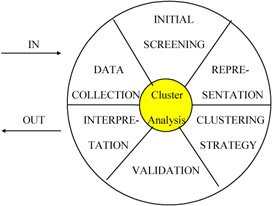
Figure 1: Clustering methodology

Data Model

Selection of Patient Attributes

In this research, the goal is to group together the records with similar attributes. A large number of variables (attributes) is not desirable to find the similarity-reduction, and selection of variables is a fundamental step in cluster analysis (Hand, 1981). In systems, i.e., PMI database, a patient is characterized by the following variables:

1. HKID number / Birth Certificate number
2. Name in English
3. Name in Chinese
4. Marital status
5. Sex
6. Date of birth
7. Age
8. Address / District code
9. Telephone number
10. Nationality
11. Religion

The values of some of these variables may change considerably over time, or they are not filled in the database. In order to determine which variables are to be chosen, three basic criteria are used: stability of the variable, accuracy of the variable, and importance of the variable. It is important to reduce the number of variables, since computer time increases dramatically with an increase in the number of variables (Anderberg, 1973). Since the HKID numbers of two records belonging to the same patient are different, or the HKIDs are missing, HKID is not a suitable variable for clustering purposes. The variables of nationality and religion are optional input to the hospital information system, and we find that over 80% of patients do not provide such information, hence nationality and religion are not suitable. The variable age is not suitable, since patients born in different months of same year may be grouped into the same age. We are left then with six variables for computing similarity:

1. Sex
2. Name in English
3. Date of birth
4. Marital status
5. District code
6. Telephone number

Furthermore, marital status, district code and telephone number are unstable variables. They often change because a patient may get married or change his/her residence and telephone number. However, these changes occur rarely, so the stability of these variables remain quite high. The variable Name in English may also be changed, but it is rare. The final variable, date of birth, will not change. Thus, we use the above six variables and use different combinations of these variables to obtain good clusters.

Data Representation, Standardization, and Weighting

Data Representation

Clustering algorithms group objects based on indices of proximity between pairs of objects. Each object is represented by a pattern or d-place vector, which indicates the d-attributes of the object. The collection of each d-place pattern forms a pattern matrix. Each row of this matrix defines a pattern and each column denotes a feature or attribute (Figure 2a). The information of the pattern matrix can be used to build a proximity matrix (Figure 2b). A proximity matrix [d(i,j)] gathers the pair-wise indices of proximity in a matrix, in which each row and column represents a pattern. A proximity index can represent either a similarity or dissimilarity. The more the ith and jth objects resemble one another, the larger the similarity index or the smaller the dissimilarity index. Only the upper triangle of the proximity matrix needs to be considered, as it is symmetric. The properties of a proximity index between the ith and kth pattern [denoted as d(i,k)] have been summarized as:

1. 1. For a dissimilarity, d(i,i) = 0, for all i.
   2. For a similarity, d(i,i) > = max d(i,k), for all i.
2. d(i,k) = d(k,i), for all (i,k).
3. d(i,k) > 0, for all (i,k).

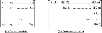
Figure 2: A pattern matrix and a proximity matrix

A C-program is written to perform the cluster analysis. As stated earlier, six attributes of each patient are used for our analysis: Sex, Date of birth, Name, Marital status, District code, and Telephone number. The HKID number is used internally for testing purposes, but not to compute clusters.

Dissimilarity Computation

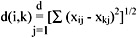
Comparison between two objects can be expressed in either similarity or dissimilarity. The Euclidean distance, a mathematical function of the distance between two objects, is used for measurement. Let [xij] be our pattern matrix, where x is the jth feature for the ith pattern. The ith pattern, which is the ith row of the pattern matrix, is denoted by the column vector xi.

xi = (xi1, xi2,.............xid)T, i = 1,2,.......,n

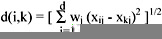
The Euclidean distance between object i and object k can then be expressed as:

As our data file consists of both ordinal and binary values, we handle it in the following way. Let the attribute of a patient be j = {1,2,3,4,5,6} equivalent to {sex, date of birth, name, marital status, district code, telephone number} respectively. For any object i or k,

if j = 1,4,5,6, (i.e., attribute = sex, marital status, district code or telephone number),

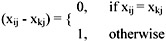
If j = 2 (i.e., attribute = date of birth),

• (xij - xkj) = the number of days between two dates of birth.

If j = 3 (i.e., attribute = name),

• (xij - xkj) = the percent of mismatched characters between two names.

The sum of these six individual values, by the definition of Euclidean distance, represents the overall dissimilarity between two objects, which forms the basic component in our proximity matrix. For example, consider the following two rows from the pattern matrix:

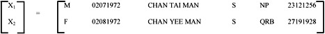
for j=1,	(d11 - d21) = 1	(Not the same sex)
for j=2,	(d12 - d22) = 31	(No. of days between date of births)
for j=3,	(d13 - d23) = 1 - 9/12 = 0.25	(% of no. of mismatch characters)
for j=4,	(d14 - d24) = 0	(Both are single)
for j=5,	(d15 - d25) = 1	(Not the same district code)
for j=6,	(d16 - d26) = 1	(Different telephone no.)

By the definition of Euclidean distance, the dissimilarity between x1 and x2 is:

• d(1,2) = [12+312+0.252+02+12+12]1/2 = 31.0494

Treatment of Missing Data

In practice, the pattern vectors can be incomplete because of errors, or unavailability of information. Jain (1988) described a simple and general technique for handling such missing values. The distance between two vectors xi and xk containing missing values is computed as follows. First, define dj between the two patterns along the jth feature:

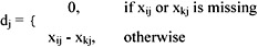
Then the distance between xi and xk is written as:

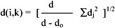
where do is the number of features missing in xi or xk or both.

If there are no missing values, then d(i,k) is the Euclidean distance. In this research, missing data is represented by "0" in the data file. Now, suppose the telephone number of patient 2 is missing (i.e., x26 = 0) in the previous example, d0 = 1

∑dj2 = 12+312+0.252+02+12+02 = 963.0625

d(1,2) = [6 / (6 - 1)] x 963.0625 = 33.9952

Data Standardization

The individual dissimilarity value for all attributes of a patient falls between 0 and 1, except the attribute of the date of birth, whose value varies from 0 to hundreds of thousands. This creates a bias in the cluster analysis towards date of birth. Normalization is performed so that the range of all measurements is 0 to 1. The standard normalization for a number, xij, can be expressed as:

where

and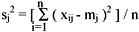

where

• xij is the actual magnitude of the variable,
• mj is the mean of all xij for attribute j, and
• sj is the standard deviation of all xij for attribute j.

Consider the previous example, let there be 100 patient records (i.e., n=100). x12 can be represented as the number of days between the date of birth and a standard date of 31121999. Therefore:

• x12 = days difference between 02071972 and 31121999 = 10039
• x22 = days difference between 02081972 and 31121999 = 10008

Now, suppose m2 = 18000, s2 = 8000, for 100 patient records:

• x12 * = (10039 - 18000) / 8000 = -0.9951
• x22 * = (10008 - 18000) / 8000 = -0.9999
• (d12 - d22) = (-0.9951) - (-0.9999) = 0.0039
• d(1,2) = [12+0.00392+0.252+02+12+12]1/2 = 1.7569

Thus, dominance of a single attribute is avoided.

Weighting

As discussed before, some attributes change more often than others over a period of time, therefore it is necessary to give higher weight to more stable attributes. Different weightings will result in different clusters. Applying the weighting factors, the Euclidean distance between object i and object k becomes:

Clustering Algorithms

Hierarchical Clustering

A hierarchical clustering is a sequence of partitions in which each partition is nested into the next partition in the sequence (Figure 3). The algorithm for hierarchical clustering starts with the disjoint clustering, which places each of the n objects in an individual cluster. The procedure of hierarchical clustering is as follows:

• Let the nxn proximity matrix be D=[d(i,j)].
• L(k) is the level of the kth clustering.
• A cluster with sequence number m is denoted as (m).
• The proximity between clusters (r) and (s) is denoted as d[(r),(s)].

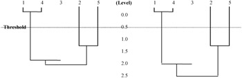
Figure 3: Hierarchical clustering

• Step 1. Begin with the disjoint clustering having level L(0)=0 and sequence number m=0.
• Step 2. Find the least dissimilar pair of cluster in the current clustering, say pair [(r),(s)], such that d[(r),(s)] = min {d[(i),(j)]}.
• Step 3. Increment the sequence number : m ← m+1.

  Merge clusters (r) and (s) into a single cluster to form the next level clustering m. Set the level of this clustering to L(m) = d[(r),(s)].

• Step 4. Update the proximity matrix, D, by deleting the rows and columns corresponding to clusters (r) and (s), and adding a row and column corresponding to the newly formed cluster.

  The proximity between the new cluster, denoted (r,s), and the old cluster (k) is defined as follows (Jain, 1988):

  • d[(k),(r,s)] = αrd[(k),(r)] + αsd[(k),(s)] +βd[(r),(s)]+ γ|d[(k),(r)] - d[(k),(s)]|

  where αr,αs, β, γ are parameters that are based on the type of hierarchical clustering.

• Step 5. If all objects are in one cluster, stop, or else go to Step 2.

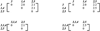
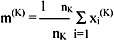
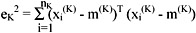
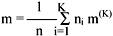
Two methods for updating the proximity matrix are provided: Single-link and compete-link. The Single-link clusters are based on connectedness and are characterized by minimum path length among all pairs of objects in the cluster. The proximity matrix is updated with d[(k),(r,s)] = min {d[(k), (r)], d[(k),(s)]}, which corresponds to αr= 0.5, αs= 0.5, β= 0 and γ =-0.5. Complete-link clusters are based on complete sub-graphs where the diameter of a complete sub-graph is the largest proximity among all proximities for pairs of objects in the sub-graph. The update of the proximity is given by d[(k),(r,s)] = max {d[(k), (r)], d[(k),(s)]}, which corresponds to αr= 0.5, αs= 0.5, β= 0 and γ = -0.5. The following example illustrates how clusters are formed among five records, with equal weighting factor of 1. Let the pattern matrix be:

The corresponding proximity matrix is:

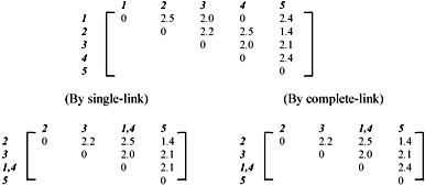
The number of clusters formed depends on the value of a threshold level.

From the above graph, it can be seen that a small threshold will return a larger number of clusters, while a large threshold will return a smaller number of clusters. In this research, we would like to obtain the most similar patient records, which implies a large number of clusters; thus it requires a smaller threshold value.

Partitional Clustering

A partitional clustering determines a partition of the n patterns into k groups or clusters, such that the patterns in a cluster are more similar to each other than to patterns in other clusters. The value of k may or may not be specified. The most commonly used partitional clustering strategy is based on the square error criterion. The objective is to obtain the partitions, which minimizes the square error for a given number of clusters. Suppose that a given set of n patterns in d dimensions has been partitioned into K clusters {C1, C2,........CK} such that cluster CK has nK patterns and each pattern is in exactly one cluster, so that:

The mean vector, or centre, of cluster CK is defined as the centroid of the cluster, or

where xi(K) is the ith pattern belonging to cluster CK. The square error for cluster CK is the sum of the squared Euclidean distances between each pattern in CK and its cluster centre m(K):

This square error is the within-cluster variation. The square error for the entire clustering containing K clusters is the sum of the within-cluster variation:

The pooled mean, m, is the grand mean vector for all the patterns:

The between-cluster variation is defined as fK2 = (m(K) - m)T(m(K) - m),

and the sum of the between-cluster variation is .

The overall square error for the entire clustering is expressed as ϕ = ϕW + ϕB. The basic idea of an iterative clustering algorithm is to start with an initial partition and assign patterns to clusters, so as to reduce the overall square error. It is clear that increasing the between-cluster scatter jB decreases the within-cluster scatter ϕW and vice verse. This general algorithm for iterative partitional clustering method is given by Gorden (1981). The partitional clustering procedure is as follows:

• Step 1. Select an initial partition with K clusters. Repeat Steps 2-5 until the cluster membership stabilizes.
• Step 2. Generate a new partition by assigning each pattern to its closest cluster centre.
• Step 3. Compute new cluster centres as the centroids of the clusters.
• Step 4. Repeat Steps 2 and 3 until an optimum value of the criterion function is formed or the total number of iteration is reached.
• Step 5. Adjust the number of clusters by merging and splitting existing clusters or by removing small clusters, or outliers.

Hybrid Clustering

In this research, we develop and use a hybrid clustering, in which the hierarchical and partitional algorithms are combined and modified to produce clustering. We compare the results of the hybrid algorithm with the other two clustering algorithms. From the output of hierarchical clustering, we can obtain different cluster combinations for a different threshold. They serve as the initialization for the partitional clustering. The hybrid clustering algorithm can be described as follows:

• Step 1. Select an initial partition from one of the results of hierarchical clustering by adjusting different threshold of the level.
• Step 2. Generate a new partition by assigning each pattern to other clusters one by one.
• Step 3. Compute new cluster centres as the centroids of the clusters, as well as the overall square error.
• Step 4. Choose the partition with the lowest value of overall square error.
• Step 5. Repeat Steps 2 – 4 for other patterns.
• Step 6. Repeat Steps 2 – 5 until an optimum value of the criterion function is found or the specified number of iteration is reached.

Refinements

As discussed before, there are several factors that affect clustering, and these need to be adjusted to obtain better results. The number of attributes is one of the factors. The higher the number of attributes, the more accurate the results will be. However, the running time will increase. There should be a tradeoff between them. The second factor is weight assignment to attributes. An attribute should not be weighted too high, since it will dominate other attributes. There should be an appropriate weighting for each attribute. Thirdly, the number of clusters chosen for initialization in partitional clustering is another factor. If the number of clusters is too small, the overall square error will be too high. But if the number of clusters is too large, the records of the same patient may distribute into different clusters. Therefore, different combinations of these factors needed to be experimented with until satisfactory results are obtained.

Results

In order to test the clustering algorithms, simulation studies involving the generation of artificial data set, for which the true structure of the data is known in advance, is used. The performance of the clustering method can then be assessed by determining the degree to which it can discover the true structure.

First Experiment

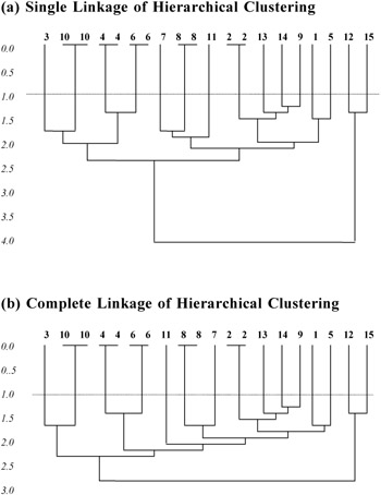
A simulated data set is used to compare the power of the three clustering algorithms. For an easy identification of duplicated records, 20 records are used, in which five of them are with repetitions. In hierarchical clustering, both the single-linkage method and the complete-linkage method are used to cluster the records. The corresponding dendrograms for both the single-linkage and complete-linkage are shown in Appendix 1. In both methods, the duplicated records are grouped, but with different subsequent formation of clusters. From the dendrograms, it can be seen that a small threshold will produce the same clustering result. The summarized results for the three algorithms are shown in Figure 4.

Algorithm	No. of cluster	mean square error		% of error		No. of iteration for convergence
		iteration	iteration	iteration	iteration
Hierarchical	5 10 15	1124 60.4 20	- - -	0 0 0	- - -	- - -
Partitional	5 10 15	109.9 40.45 33.4	91.55 38.9 30.25	40 60 100	40 60 80	>500000 >500000 >500000
Hybrid	5 10 15	227.05 36.8 20	201.55 30.1 20	0 0 0	0 0 0	<5000 <5000 <100

Figure 4: The best results for the three clustering algorithms with 20 input records

From Figure 4, it can be seen that the mean square error of hierarchical clustering is larger than that of partitional clustering. However, the percentage of error in hierarchical clustering is smaller than that of partitional clustering when the number of iteration is small. The result of partitional clustering can further be improved by increasing the number iteration so as to reduce the mean square error, and percentage of error. At the same time, it increases the time for convergence. Hybrid clustering combines the advantages from both the hierarchical clustering and partitional clustering. With a good choice of threshold, records are well structured into clusters by the initializing hierarchical clustering. Then the structure is further re-organized in order to reduce the mean square error by the following partitional clustering. As the choice of initial number of cluster is first determined by the hierarchical part, number of iteration can highly be reduced to get the local minimum or even the global minimum. The rate of convergence is much faster than that of partitional clustering.

Second Experiment

A second simulation study is also performed, but with a much larger data set. 100 records are used in which 10% are with repetition. The summarized results from the hierarchical clustering, partitional clustering and hybrid clustering are shown in Figures 5 to 7, respectively.

As can be seen in Figure 5, the best solution is obtained without any error by the hierarchical clustering (number of cluster=90). It forms the initialization of number of clusters in hybrid clustering. The structure of the result can further be reduced with a decrease in mean square error by increasing the number of iteration (number of cluster=88 in Figure 7). In Figure 6, the best solution is obtained when the number of clusters is 93 with 10% of error. This solution is only the local minimum with 1000 iterations. A global minimum appears when the number of iteration is increased so that there is no error. The rate of convergence is much lower in partitional clustering than the hybrid clustering. As seen in Figure 7, the hybrid clustering converges after 500 iterations, but the partitional clustering still oscillates.

Threshold	No. of cluster	Mean square error	% of error
0.5	90	100	0
1	90	100	0
1.5	25	865	0
2	2	71249	0
3.5	2	72215	0

Figure 5: Summarized result for the hierarchical clustering with 100 input records

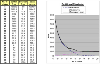
Figure 6: Summarized result for the partitional clustering with 100 input records

Algorithm	Threshold	No. of cluster	Mean square error
			No. of iteration
			0	100	200	500	1000
Hybrid	0.5	90	100	95.2	94.4 (reduce to 88 clusters)	94.4 (reduce to 88 clusters)	94.4 (reduce to 88 clusters)
	1	90	100	95.2	94.4 (reduce to 88 clusters)	94.4 (reduce to 88 clusters)	94.4 (reduce to 88 clusters)
	1.5	25	865	824	806	794	794
	2	2	712 49	70867	70584	70151.9	70151.9
Partitional		90		132.01	132.01	132.01	111.88
		25		596.71	596.71	596.71	570.71
		2		72105.97	72105.97	72105.97	7274.97

Figure 7: Summarized result for the hybrid clustering with 100 input records

Comparison

The primary step in hierarchical clustering is to group those records with high similarity. Once the records are grouped into any cluster, they will not be further considered individually. The similarity of the whole cluster will then be compared with other records to form a much larger cluster, if necessary. On the other hand, partitional clustering considers all the records every time and tries to group them into different clusters with the total least difference among the elements within clusters. It needs a very long time to re-structure the clustering before a fairly good result can be obtained. The combination of the two algorithm forms the hybrid clustering algorithm. It tries to reduce the time of iteration required in partitional clustering by constructing a quite good starting structure using hierarchical clustering first. The objective is then achieved by further searching the global minimum value of the overall mean square error.

Future Trends

The present research has the following limitations, and thus the research can be extended to eliminate these limitations. The weights we used are somewhat arbitrary. More simulation studies may be needed to determine the appropriate weights on the training data set. Secondly, the threshold value was arbitrarily chosen in this research, since we are aware of the actual data. In a real life situation, we do not know what percentage of patients have multiple records. The threshold value can also be estimated based on the error history of patient records. Thus, future researchers may need to repeat the experiment with different threshold values in order to determine the best one. Finally, the selection of the attributes of patient records needs consideration. This research can be extended to determine the appropriate set of attributes, by considering the knowledge of the hospital staff and also by using other algorithms (such as genetic algorithms) that will help determine an optimal set of attributes. Genetic algorithms, developed based on biological evolution, are widely used to solve optimization problems in data mining techniques (Berson & Smith, 1997). By using genetic algorithms, various combinations of attributes will be considered and evaluated for superiority in identifying records of the same patient. In this research, we considered clustering algorithms as a data mining technique. Future research should consider other techniques, such as association rules, use of entropy, etc. (Han & Kamber, 2001), and compare the results with clustering. Entropy is an information-based concept that can be used to partition a data set based on an attribute, resulting in a hierarchical discretization. Another extension to the present research can be done by employing other clustering algorithms proposed, such as those by Guha et al. (2000, 2001), and comparing the results. These issues are left for future investigation.

Conclusion

In this research, we illustrated the use of data mining techniques, particularly clustering algorithms, to identify duplicate patient records in Hospital Information Systems. The reasons for errors in patient data are wrong data entry, insufficient information provided by the patient, improper identity of the patients (in the case of tourists in Hong Kong), etc. The clustering algorithms are used in this research to cluster all the records of each patient together, so that high quality data records of each patient can be maintained. The importance of this research cannot be over-emphasized because of the fact that wrongly grouped records or ungrouped records of a patient will give rise to inaccurate or missing information about the patient's medical history, which will further lead to erroneous conclusions by the doctors.

We used three clustering algorithms: hierarchical, partitioned, and hybrid that combines the other two. Our results show that Hybrid algorithm gave more accurate groupings compared to the other algorithms, and result was obtained faster (fewer iterations). In the hybrid algorithm, by minimizing the total squared error, we could obtain the best clustering. In this research, we demonstrated that data mining technique could be used to detect data duplications by experimenting on a smaller set of data. However, this procedure can be adapted to any size data set, since we observed in our research that the hybrid algorithm ran a thousand times faster than conventional partitional clustering algorithms. We used six attributes of patient data to cluster the patient records — Sex, Date of birth, Name, Marital status, District, and Telephone number — as the basis for computing similarity of patient records. We also used some weights to these variables in computing similarity, which were based on simulation.

References

Anderberg, M. R. (1973). Cluster analysis for applications. New York: Academic Press.

Backer, E. (1995). Computer-assisted reasoning in cluster analysis. New York: Prentice Hall.

Berson, A., & Smith, S. (1997). Data warehousing, data mining, & OLAP. McGraw-Hill.

Diday, E. (1994). New approaches in classification and data analysis. New York: Springer-Verlag.

Everitt, B. S. (1974). Cluster analysis. London: E. Arnold.

Gordon, A.D. (1981). Classification: Methods for the exploratory analysis of multivariate data. London: Chapman and Hall.

Guha, S., Rastogi, R., & Shim, K. (2000). ROCK: a robust clustering algorithm for categorical attributes. Information Systems, 25 (5), 345–66.

Guha, S., Rastogi, R., & Shim, K. (2001). CURE: An efficient clustering algorithm for large databases. Information Systems, 26 (1), 35–58.

Han, J., & Kamber, M. (2001). Data mining: Concepts and techniques. Morgan Kaufmann Publishers.

Hand, D.J. (1981). Discrimination and classification. New York: J. Wiley.

Hubert, L.J. (1995). Clustering and classification. Singapore: World Scientific.

Jain, A.K. (1988). Algorithms for clustering data. NJ: Prentice Hall.

McLachlan, G. J, (1988), Mixture models: Inference and applications to clustering". NY: M. Dekker.

Modell, M.E. (1992). Data analysis, Data modeling, and classification. New York: McGraw-Hill.

Rencher, A.C. (1995). Methods of multivariate analysis. New York: Wiley.

Sholom, M. W. (1991). Computer systems that learn. CA: Morgan Kaufmann.

Spath, H.. (1980). Cluster analysis algorithms for data reduction and classification of objects. New York: Halsted Press.

Willett, P. (1987). Similarity and clustering in chemical information systems. New York: J. Wiley.

Appendix 1 Simulation Result Dendrograms for Single Link Output vs Complete Link Output