Hack 75. Share Your GRASS Maps with the World


Export your carefully crafted GIS layers into human-compatible formats.
If you've worked through the GRASS hacks in this book, you might have noticed a standard finale: "Now see [Hack #75] to export your maps to an image file." Having got this far, congratulations! Now the world can know of your triumphant ascent of the GRASS learning curve.
The r.out set of GRASS functions provides many ways to export your raster layers into different GIS-compatible formats, such as ESRI's ArcInfo, binary vector format, etc. However, the most useful formats to share map data inPNG for viewing on the Web, or PostScript for print publicationboth involve some fiddling.
6.13.1. Publish Raster Maps as PNG Images
In the simplest case, you might just have a raster layer in GRASS that you want to export as a PNG image. r.out.png is ideal for these purposes:
GRASS:~ > r.out.png in=nations out=nations.png
rows = 2250, cols = 4500
Converting nations... 96%
Done.
You should note that r.out.png, like most GRASS raster functions, only operates on the current region. Be sure to run g.region rast=... first if you want to export the whole raster layer.
6.13.2. Publish PNG Images via the Display Monitor
If you have a whole set of different layers you want to export together, it's better to use the PNG display driver that comes with GRASS. This works just like writing to an X monitor with d.mon, except that it's writing directly to a .png file.
GRASS:~ > d.mon start=PNG
PNG: GRASS_TRUECOLOR status: FALSE
PNG: collecting to file: map.png,
 GRASS_WIDTH=640, GRASS_HEIGHT=480
Graphics driver [PNG] started
GRASS:~ > d.rast eco
 100%
GRASS:~ > d.vect borders type=boundary color=black
GRASS:~ > d.mon stop=PNG
Monitor 'PNG' terminated
The disadvantage of this approach is that you can't see the image while you're creating it, and it can be annoying to have to repeat a long sequence of command-line actions if you make a small mistake. This is where d.save will save you.
As discussed in [Hack #69], d.save -c prints the list of commands that were used to generate the current contents of the display monitor to its standard output. You can use shell redirection to pipe this list to a file and then manually add the d.mon start=png line to the beginning and the d.mon stop=png line to the end. The result is a shell script that will generate your PNG. You can run it directly from the GRASS shell and tweak the lines until you're quite happy with the results.
By default, the PNG monitor generates a 256-color image 640 pixels wide and 480 pixels high and stores it in a file called map.png, but we can alter that outcome with a variety of environment variables. The following commands export the map described in [Hack #69] with a black background to an 800 600 pixel True Color PNG file called western_europe.png:
GRASS:~ > export GRASS_WIDTH=800
GRASS:~ > export GRASS_HEIGHT=600
GRASS:~ > export GRASS_TRUECOLOR=TRUE
GRASS:~ > export GRASS_BACKGROUNDCOLOR=000000
GRASS:~ > export GRASS_PNGFILE=western_europe.png
GRASS:~ > d.mon start=PNG
PNG: GRASS_TRUECOLOR status: TRUE
PNG: collecting to file: western_europe.png,
 GRASS_WIDTH=800, GRASS_HEIGHT=600
 Graphics driver [PNG] started
GRASS:~ > sh ./europe.sh
 100%
GRASS:~ > d.mon stop=PNG
Monitor 'PNG' terminated
GRASS:~ > d.mon select=x0
The last d.mon command reselects our original X11 monitor, so that any further display commands are sent there, rather than to the now-closed PNG monitor. You can now view the PNG file in an ordinary image viewer or upload it to the Web to share with your friends and colleagues.
|

6.13.3. Publish GRASS Maps as PostScript Files
Generating PostScript images from GRASS isn't quite as straightforward as generating PNGs, but the results will often look a lot nicer. The ps.map utility provided for this purpose is classic GRASS: it's flexible, powerful, and utterly arcane. ps.map is driven by a "little language" for display scripting that, when fed to GRASS, will generate PostScript code. With ps.map, you can add color tables, legends, custom fonts, and scale indicators, all the visual trappings of professional looking print cartography.
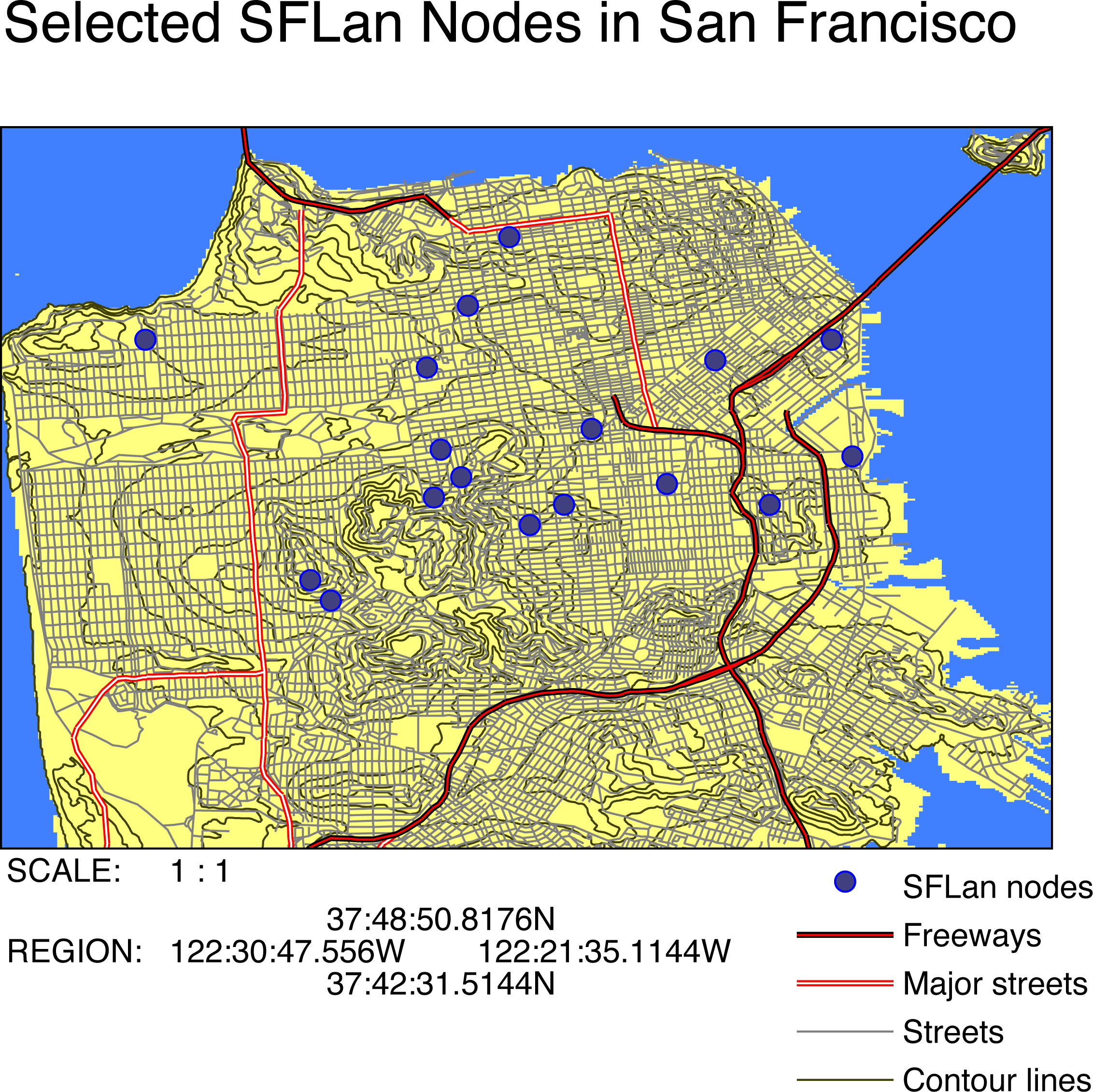
Figure 6-46 shows a PostScript map of selected nodes from SFLan, a community wireless network based in San Francisco. The map was made with TIGER/Line street data, National Elevation Data obtained from the USGS SDDS, and, of course, ps.map. The contour lines were generated in the fashion described in [Hack #73] .
Figure 6-46. A map of San Francisco generated with ps.map
Example 6-1 shows the set of ps.map commands used to tell GRASS to generate Figure 6-46.
Example 6-1. sf_tiger.txt: ps.map commands used to generate Figure 6-46
 raster dem


 vpoints sflan

 label SFLan nodes

 color blue

 fcolor 64 64 128

 symbol basic/circle

 size 10

 end


 vlines tiger

 where CFCC ~ 'A1'

 label Freeways

 color red

 width 1

 hcolor black

 hwidth 1

 end


 vlines tiger

 where CFCC ~ 'A3' OR CFCC ~ 'A2'

 label Major streets

 color white

 width 1

 hcolor red

 hwidth 1

 end


 vlines tiger

 where CFCC ~ 'A5' or CFCC ~ 'A4'

 label Streets

 color grey

 width 1

 end


 vlines sfcontour

 label Contour lines

 color 64 64 0

 end


 vlegend

 where 6 0

 fontsize 16

 end


 mapinfo

 where 0 0

 fontsize 16

 end


 header

 file sf_tiger_hdr.txt

 fontsize 28

 end
The raster command in line 1 of sf_tiger.txt draws the digital elevation model of San Francisco as a raster base layer, which had been previously colored to distinguish land and water areas. Lines 3-9 draw the location of SFLan nodes from the sflan vector layer, with circles drawn in blue and filled with a darker shade of blue. Lines 11-18 introduce a vlines block, which draws a portion of a layer called tiger. The where command in line 12 filters the vectors to draw only those that have a Census Feature Class Code (CFCC) attribute matching A1, which corresponds to limited-access highways. (The CFCC attribute is just a property of the particular data set used to draw the map.) These features are given the label "Freeways" and drawn in a red line 1 pixel wide, with a black highlight 1 pixel wide on either side. Major streets and ordinary streets are given corresponding treatment in lines 20-34. In lines 36-39, the contour lines from the sfcontour vector layer are drawn in brown. The legend and map information are placed in lines 41-49, and lines 51-54 display the contents of a text file called sf_tiger_hdr.txt across the header of the map, in 28-point type.
|
ps.map is run in the following fashion:
GRASS:~ > ps.map input=sf_tiger.txt output=sf_tiger.ps
If you don't have a PostScript viewer, some free alternatives are available in [Hack #28] . If, for whatever reason, you prefer Encapsulated PostScript, ps.map will generate that instead, with the -e option. From there, you can use a tool like the epstopdf program that ships with GhostScript to convert PostScript or EPS to PDF, for example.
One drawback with ps.map is that it can only read one raster layer into a PostScript image, unless you're using three rasters to make RGB color composites. If you want to display the results of layering more than one raster image togetherfor example, the topographical height field as a transparent layer over a DRG street map [Hack #72] you have to first combine them into one raster layer, perhaps by using r.patch or r.composite.
As PostScript is a vector format, vector display is where it really shines, and you can layer as many vectors into your PostScript document as you like. ps.map has different vector options for importing shapes, lines, and points. However, the parameters are more or less the same for each vector option.
Obviously, with a tool as powerful as ps.map, we can only offer the outlines of its general functionality, and we strongly recommend perusing the documentation if you're interested in publishing your maps to the world this way.
Mapping Your Life
- Hacks 1-13
- Hack 1. Put a Map on It: Mapping Arbitrary Locations with Online Services
- Hack 2. Route Planning Online
- Hack 3. Map the Places Youve Visited
- Hack 4. Find Your House on an Aerial Photograph
- Hack 5. The Road Less Traveled by in MapQuest
- Hack 6. Make Route Maps Easier to Read
- Hack 7. Will the Kids Barf?
- Hack 8. Publish Maps of Your Photos on the Web
- Hack 9. Track the Friendly Skies with Sherlock
- Hack 10. Georeference Digital Photos
- Hack 11. How Far? How Fast? Geo-Enabling Your Spreadsheet
- Hack 12. Create a Distance Grid in Excel
- Hack 13. Add Maps to Excel Spreadsheets with MapPoint
Mapping Your Neighborhood
- Hacks 14-21
- Hack 14. Make Free Maps of the United States Online
- Hack 15. Zoom Right In on Your Neighborhood
- Hack 16. Who Are the Neighbors Voting For?
- Hack 17. Map Nearby Wi-Fi Hotspots
- Hack 18. Why You Cant Watch Broadcast TV
- Hack 19. Analyze Elevation Profiles for Wireless Community Networks
- Hack 20. Make 3-D Raytraced Terrain Models
- Hack 21. Map Health Code Violations with RDFMapper
Mapping Your World
- Hacks 22-34
- Hack 22. Digging to China
- Hack 23. Explore David Rumseys Historical Maps
- Hack 24. Explore a 3-D Model of the Entire World
- Hack 25. Work with Multiple Lat/Long Formats
- Hack 26. Work with Different Coordinate Systems
- Hack 27. Calculate the Distance Between Points on the Earths Surface
- Hack 28. Experiment with Different Cartographic Projections
- Hack 29. Plot Arbitrary Points on a World Map
- Hack 30. Plot a Great Circle on a Flat Map
- Hack 31. Plot Dymaxion Maps in Perl
- Hack 32. Hack on Base Maps in Your Favorite Image Editor
- Hack 33. Georeference an Arbitrary Tourist Map
- Hack 34. Map Other Planets
Mapping (on) the Web
- Hacks 35-46
- Hack 35. Search Local, Find Global
- Hack 36. Shorten Online Map URLs
- Hack 37. Tweak the Look and Feel of Web Maps
- Hack 38. Add Location to Weblogs and RSS Feeds
- Hack 39. View Your Photo Thumbnails on a Flash Map
- Hack 40. Plot Points on a Spinning Globe Applet
- Hack 41. Plot Points on an Interactive Map Using DHTML
- Hack 42. Map Your Tracklogs on the Web
- Hack 43. Map Earthquakes in (Nearly) Real Time
- Hack 44. Plot Statistics Against Shapes
- Hack 45. Extract a Spatial Model from Wikipedia
- Hack 46. Map Global Weather Conditions
Mapping with Gadgets
- Hacks 47-63
- How GPS Works
- Hack 47. Get Maps on Your Mobile Phone
- Hack 48. Accessorize Your GPS
- Hack 49. Get Your Tracklogs in Windows or Linux
- Hack 50. The Serial Port to USB Conundrum
- Hack 51. Speak in Geotongues: GPSBabel to the Rescue
- Hack 52. Show Your Waypoints on Aerial Photos with Terrabrowser
- Hack 53. Visualize Your Tracks in Three Dimensions
- Hack 54. Create Your Own Maps for a Garmin GPS
- Hack 55. Use Your Track Memory as a GPS Base Map
- Hack 56. Animate Your Tracklogs
- Hack 57. Connect to Your GPS from Multiple Applications
- Hack 58. Dont Lose Your Tracklogs!
- Hack 59. Geocode Your Voice Recordings and Other Media
- Hack 60. Improve the Accuracy of Your GPS with Differential GPS
- Hack 61. Build a Map of Local GSM Cells
- Hack 62. Build a Car Computer
- Hack 63. Build Your Own Car Navigation System with GpsDrive
Mapping on Your Desktop
- Hacks 64-77
- Hack 64. Mapping Local Areas of Interest with Quantum GIS
- Hack 65. Extract Data from Maps with Manifold
- Hack 66. Java-Based Desktop Mapping with Openmap
- Hack 67. Seamless Data Download from the USGS
- Hack 68. Convert Geospatial Data Between Different Formats
- Hack 69. Find Your Way Around GRASS
- Hack 70. Import Your GPS Waypoints and Tracklogs into GRASS
- Hack 71. Turn Your Tracklogs into ESRI Shapefiles
- Hack 72. Add Relief to Your Topographic Maps
- Hack 73. Make Your Own Contour Maps
- Hack 74. Plot Wireless Network Viewsheds with GRASS
- Hack 75. Share Your GRASS Maps with the World
- Hack 76. Explore the Effects of Global Warming
- Conclusion
- Hack 77. Become a GRASS Ninja
Names and Places
- Hacks 78-86
- Hack 78. What to Do if Your Government Is Hoarding Geographic Data
- Hack 79. Geocode a U.S. Street Address
- Hack 80. Automatically Geocode U.S. Addresses
- Hack 81. Clean Up U.S. Addresses
- Hack 82. Find Nearby Things Using U.S. ZIP Codes
- Hack 83. Map Numerical Data the Easy Way
- Hack 84. Build a Free World Gazetteer
- Hack 85. Geocode U.S. Locations with the GNIS
- Hack 86. Track a Package Across the U.S.
Building the Geospatial Web
- Hacks 87-92
- Hack 87. Build a Spatially Indexed Data Store
- Hack 88. Load Your Waypoints into a Spatial Database
- Hack 89. Publish Your Geodata to the Web with GeoServer
- Hack 90. Crawl the Geospatial Web with RedSpider
- Hack 91. Build Interactive Web-Based Map Applications
- Hack 92. Map Wardriving (and other!) Data with MapServer
Mapping with Other People
- Hacks 93-100
- Hack 93. Node Runner
- Hack 94. Geo-Warchalking with 2-D Barcodes
- Hack 95. Model Interactive Spaces
- Hack 96. Share Geo-Photos on the Web
- Hack 97. Set Up an OpenGuide for Your Hometown
- Hack 98. Give Your Great-Great-Grandfather a GPS
- Hack 99. Map Your Friend-of-a-Friend Network
- Hack 100. Map Imaginary Places
EAN: 2147483647
Pages: 172
