Getting the Words Right

Worksheets are not all numbers, of course, so Office Excel 2007 includes several features to help make typing and editing text easier. AutoCorrect helps you fix common typing errors even before they become spelling problems. For the rest of the words in your worksheets, the spelling checker helps make sure you've entered your text according to Webster. You might even be able to get AutoComplete to do some of the typing for you. And finally, the Research, Thesaurus, and Translate features lend some real clout in your quest for perfect prose.

Fixing Errors As You Type

Perhaps you have to stop and think "i before e except after c" every time you type receive. Perhaps you're a blazing typist who constantly hits the second letter of a capitalized word before the Shift key snaps back. The Excel AutoCorrect feature helps fix many common typing and spelling errors on the fly. Click the Microsoft Office Button, Excel Options, and in the Proofing category, click the AutoCorrect Options button to display the AutoCorrect dialog box shown in Figure 8-38.

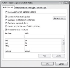
Figure 8-38: You can add your most common typing errors to the AutoCorrect dialog box.

Note 

AutoCorrect works when entering text in cells, formulas, text boxes, on-worksheet controls, and chart labels. AutoCorrect does not work when entering text in dialog boxes.

The AutoCorrect tab in the AutoCorrect dialog box contains the following options:

• Show Auto Correct Options Buttons Controls the display of the smart tag action menu when Excel detects an error, listing actions you can perform on the affected cell.

• Correct TWo INitial CApitals If a word contains both uppercase and lowercase characters, checks that only one capital letter appears at the beginning of the word. If not, Excel changes subsequent uppercase characters to lowercase. If a word is all caps, Excel leaves it alone (assuming that this was intentional). AutoCorrect does not attempt to modify "mid-cap" words like AutoCorrect, probably because of their increasing usage.

• Capitalize First Letter Of Sentences Makes sure you use "sentence case" (even if your sentences aren't grammatically correct), based on the position of periods.

• Capitalize Names Of Days Recognizes days and applies initial caps. This does not work on abbreviations like Sat.

• Correct Accidental Use Of cAPS LOCK Key Scans for this kind of random Shift-key mistake.

• Replace Text As You Type Controls the application of the replacement list at the bottom of the dialog box, which lists a number of common replacement items. You can add your own grammatical faux pas to this list using the Replace and With text boxes and the Add button.

In addition to correcting common typing errors such as replacing adn with and, AutoCorrect also provides a few useful shortcuts in its replacement list. For example, instead of searching for the right font and symbol to add a copyright mark, you can type (c), and AutoCorrect replaces it with ©.

All these AutoCorrect options use specific rules of order. They use similar, logical methods to determine your real meaning. But don't assume that AutoCorrect (or the spelling checker) knows what you mean. Always proofread important work.

Note 

If you have other Microsoft Office programs installed, anything you add to the AutoCorrect list in Excel will also appear in other Office programs' AutoCorrect lists.

Typing Internet and Network Addresses

We like to refer to this feature as AutoAutoFormat. The AutoFormat As You Type tab in the AutoCorrect dialog box (shown in Figure 8-33 on page 220) offers the Internet And Network Paths With Hyperlinks option under Replace As You Type. This converts a string recognized as a valid uniform resource locator (URL) or network path into an active hyperlink. As you finish typing it, you can click it immediately to go there.

For more about formatting as you type, see "Extending Existing Formatting" on page 219.

Using Custom AutoCorrect Smart Tags

The Smart Tags tab in the AutoCorrect dialog box shown in Figure 8-39 is the repository for customized smart tags. Excel comes with several of them, and you can download additional smart tags as they become available on the Microsoft Office Online Web site (http://office.microsoft.com/).

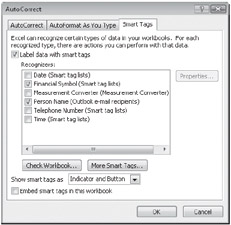
Figure 8-39: The Smart Tags tab in the AutoCorrect dialog box is the control center for all your smart tag needs.

The following smart tag options are available in the AutoCorrect dialog box:

• Recognizers Describes the currently installed smart tags in terms of what they look for as you type and includes items such as Date, Financial Symbol, Person Name (e-mail recipient), Telephone Number, and Time. Figure 8-40 shows the smart tag action menus for Financial Symbols and Person Name.

• Check Workbook Applies the selected recognizers to existing data in your workbook, letting you add smart tags to existing workbooks. If you do, you need to select the Embed Smart Tags In This Workbook check box.

• More Smart Tags Adds custom recognizers found on the Office Update Web site to the Recognizers list. You'll need to be connected to the Internet.

• Show Smart Tags As Displays smart tags. Select Indicator And Button (the default), Button Only, or None. Smart tags ordinarily appear as a small triangle in the lower-right corner of the cell (the indicator); in addition, an icon appears when you rest your pointer on the cell (the button).

• Embed Smart Tags In This Workbook Permanently attaches smart tags to previously recognized data.

• Properties Tells you more about the smart tag you selected in the Recognizers list. You'll need to be connected to the Internet for this one.

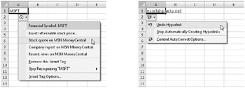
Figure 8-40: Excel includes built-in custom smart tag action menus for stock-ticker symbols and e-mail addresses, among other types of data.

Letting Excel Help with Typing Chores

Often when entering a large amount data in one sitting, you end up typing the same entries repeatedly. The AutoComplete feature cuts down the amount of typing you need to do. It also increases the accuracy of your entries by partially automating them. AutoComplete is on by default, but you can turn it off by clicking the Microsoft Office Button, Excel Options, and the Advanced category and then clearing the Enable AutoComplete For Cell Values check box in the Editing Options area.

When you begin typing a cell entry, AutoComplete scans all the entries in the same column and, as each character is typed, determines whether the column contains a possible match. (This works only when you are typing in a cell adjacent to other entries.) For example, in Figure 8-41, as soon as we typed Y in cell A14, AutoComplete finished the entry with the unique match found in the same column: Young, Rob. The text added by AutoComplete is highlighted, so you can either continue typing, if that wasn't your intended entry, or press Enter or an arrow key to accept the completion and move to another cell.

Figure 8-41: Type enough letters to match an existing entry, and AutoComplete finishes it for you. As shown on the right, keep typing to override AutoComplete.

AutoComplete matches only exact cell entries, not individual words in a cell. For example, if you begin typing Tony in column A of the worksheet, AutoCorrect doesn't intervene, because it is not an exact match for any existing entry. Wisely, AutoComplete does not work when you're editing formulas.

Instead of typing, you can click Pick From Drop-Down List on the shortcut menu to select an existing entry from the same column. To do so, right-click a cell, and click Pick From Drop-Down List in the shortcut menu, as shown in Figure 8-42. After Excel displays the list, click the entry you want, and Excel enters it in the cell. Of course, you can't add new entries this way, as we did in Figure 8-41; only existing entries in the same column are available in the list.

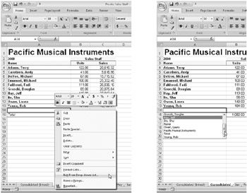
Figure 8-42: Right-click the cell directly below a list, and click Pick From Drop-Down List to display a list of unique entries in the column.

Inside Out-Create Your Own Typing Shorthand

You can use AutoCorrect to monitor your own common typing errors and create your own typing shortcuts. Click the Microsoft Office Button, Excel Options, and then click the AutoCorrect Options button in the Proofing category. Add your shorthand entries in the Replace Text As You Type area on the AutoCorrect tab. (Figure 8-38 on page 227 shows the AutoCorrect dialog box.) Type the characters you want to use as the shorthand "code" in the Replace box, then type the characters with which you want to replace them in the With box, and finally click Add. For example, you can type MS in the Replace box and then type Microsoft Corporation in the With box. Thereafter, each time you type MS, Excel replaces it with the words Microsoft Corporation. Make sure you choose unique codes; otherwise, Excel might apply AutoCorrect to entries you don't want changed.

Cheking Yer Speling

Click the Review tab on the Ribbon, and then click Spelling to check the spelling of an entire worksheet or any part of it. If Excel finds any suspect words, the Spelling dialog box shown in Figure 8-43 appears. Keep the following tips in mind when using the spelling checker:

• If you select a single cell, Excel checks the entire worksheet, including all cells, comments, Excel graphic objects, and page headers and footers.

• If you select more than one cell, Excel checks the selected cells only.

• If the formula bar is active, Excel checks only its contents.

• If you select words that are within the formula bar, Excel checks the selected words only.

• If the range you select for checking the spelling contains hidden or outlined cells that are not visible, Excel checks these as well.

• Cells that contain formulas are not checked.

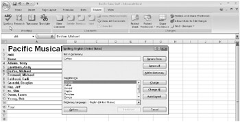
Figure 8-43: Use the Spelling dialog box to review your text and add often-used words to your dictionary.

Click Options in the Spelling dialog box to display the Excel Options dialog box. Click the Proofing category, shown in Figure 8-44. Here you can access the AutoCorrect dialog box, choose dictionaries in different languages, and select special options such as the Ignore Internet And File Addresses check box.

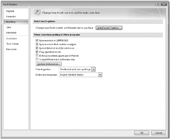
Figure 8-44: Gain more control over spelling with the Proofing tab in the Excel Options dialog box.

Note 

You can press F7 to instantly begin checking the spelling.

Research Resources

Besides Spelling, the other three buttons in the Proofing group on the Review tab-Research, Thesaurus, and Translate-provide some real horsepower when you are ready to invest time in the word play accompanying your numeric adventures. Perhaps Excel is not the most efficient way to learn a foreign language, but the Translate feature is certainly intriguing, especially if you work with international customers or co-workers. Clicking any of these three buttons displays a task pane docked to the right side of the screen, as shown in Figure 8-45. Note that only the Research button is a toggle-clicking it a second time closes the task pane. The other two buttons change what appears within the task pane.

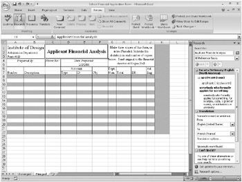
Figure 8-45: The Research, Thesaurus, and Translate buttons on the Review tab open a task pane.

The cell or range selected when you open the task pane automatically appears in the Search For box when you click one of the buttons, and any search results appear in the main area of the task pane. If you already have the task pane open and you want to change the search text, you can either type it or press Alt while clicking a cell containing the text you want, which then appears in the Search For box.

The second box under Search For is a drop-down list that lets you narrow your search to particular resources, as shown in Figure 8-46. Note, however, that when you click the Research button on the Ribbon, the default search is All Reference Books, which also includes the results that would be returned by clicking Thesaurus or Translate. If you scroll to the bottom of the search results, you'll find these categories, plus a Can't Find It? category, offering additional options. As you try different searches in the task pane, click the Back and Next buttons (a. k. a. Previous Search and Next Search) to peruse the various search results.

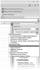
Figure 8-46: You can narrow your search to use specific resources.

You can alter the contents of the drop-down list shown in Figure 8-46 by clicking Research Options, located at the bottom of the task pane, which displays the Research Options dialog box shown in Figure 8-47. Here you can add or remove places to look from the list, update the available options, and specify parental controls, if you are logged on as an administrator. For details on a particular service, select it, and click the Properties button.

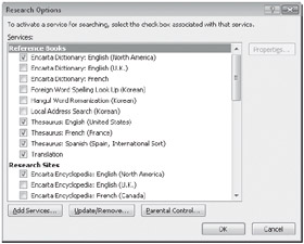
Figure 8-47: Specify the research resources available using the Research Options dialog box.

At the bottom of the task pane is a Get Updates To Your Services link, which connects you to the Microsoft Office Online Web site where Excel then checks to see whether there are any updates to existing services or any new services available that you can add to your research options.

Inside Out-Task Pane Tricks

You can reposition or resize the task pane by clicking the small arrow next to the Close button and choosing the appropriate command. Clicking the Move command changes the cursor to a four-headed arrow, letting you drag the task pane away from its "docked" position on the right side of the screen. You can let it float above the workspace or dock it on the left side if you prefer. After clicking the Size command, drag the mouse (you don't even need to click) to reposition the border of the task pane to make it wider, up to half the screen width when docked. Click when the size of the task pane is to your liking.

In actuality, you don't need these commands at all. You can drag a task pane away from the dock by its title bar at any time without using the Move command, just as you can drag the inside border of a docked task pane without using the Size command. You can drag the borders of the undocked task pane with impunity, making it as large as you like. To restore a floating task pane to its previous docked configuration, double-click its title bar. To remove a task pane from view, click the Close button in the upper-right corner of the task pane.