Details

Missing Values

Observations with missing values for any variable listed in the MODEL or POPULATION statement are omitted from the analysis.

If the WEIGHT variable for an observation has a missing value, the observation is by default omitted from the analysis. You can modify this behavior by specifying the MISSING= option in the MODEL statement. The option MISSING= value sets all missing weights to value and all missing cells to value . The option MISSING=SAMPLING causes all missing cells in a contingency table to be treated as sampling zeros.

Any observation with nonpositive weight is also, by default, omitted from the analysis. If it has zero weight, then you can specify the ZERO= option in the MODEL statement.

Input Data Sets

Data to be analyzed by PROC CATMOD must be in a SAS data set containing one of the following:

• raw data values (variable values for every subject)

• frequency counts and the corresponding variable values

• response function values and their covariance matrix

If you specify a WEIGHT statement, then PROC CATMOD uses the values of the WEIGHT variable as the frequency counts. If the READ function is specified in the RESPONSE statement, then the procedure expects the input data set to contain the values of response functions and their covariance matrix. Otherwise, PROC CATMOD assumes that the SAS data set contains raw data values.

Raw Data Values

If you use raw data, PROC CATMOD first counts the number of observations having each combination of values for all variables specified in the MODEL or POPULATION statements. For example, suppose the variables A and B each take on the values 1 and 2, and their frequencies can be represented as follows .

	A=1	A=2
B=1	2	1
B=2	3	1

The SAS data set Raw containing the raw data might be as follows.

Observation	A	B
1	1	1
2	1	1
3	1	2
4	1	2
5	1	2
6	2	1
7	2	2

And the statements for PROC CATMOD would be

  proc catmod data=Raw;   model A=B;   run;  

For discussions of how to handle structural and random zeros with raw data as input data, see the 'Zero Frequencies' section on page 888 and Example 22.5 on page 919.

Frequency Counts

If your data set contains frequency counts, then use the WEIGHT statement in PROC CATMOD to specify the variable containing the frequencies. For example, you could create the Summary data set as follows.

  data Summary;   input A B Count;   datalines;   1 1 2   1 2 3   2 1 1   2 2 1   ;  

In this case, the corresponding statements would be

  proc catmod data=Summary;   weight Count;   model A=B;   run;  

The data set Summary can also be created from data set Raw by using the FREQ procedure:

  proc freq data=Raw;   tables A*B / out=Summary;   run;  

Inputting Response Functions and Covariances Directly

If you want to read in the response functions and their covariance matrix, rather than have PROC CATMOD compute them, create a TYPE=EST data set. In addition to having one variable name for each function, the data set should have two additional variables: _TYPE_ and _NAME_ , both character variables of length 8. The variable _TYPE_ should have the value 'PARMS' when the observation contains the response functions; it should have the value 'COV' when the observation contains elements of the covariance matrix of the response functions. The variable _NAME_ is used only when _TYPE_ =COV, in which case it should contain the name of the variable that has its covariance elements stored in that observation. In the following data set, for example, the covariance between the second and fourth response functions is 0.000102.

  data direct(type=est);   input b1-b4 _type_ $ _name_ .;   datalines;   0.590463   0.384720   0.273269   0.136458   PARMS   .   0.001690   0.000911   0.000474   0.000432   COV     B1   0.000911   0.001823   0.000031   0.000102   COV     B2   0.000474   0.000031   0.001056   0.000477   COV     B3   0.000432   0.000102   0.000477   0.000396   COV     B4   ;  

In order to tell PROC CATMOD that the input data set contains the values of response functions and their covariance matrix,

• specify the READ function in the RESPONSE statement

• specify _F_ as the dependent variable in the MODEL statement

For example, suppose the response functions correspond to four populations that represent the cross-classification of two age groups by two race groups. You can use the FACTORS statement to identify these two factors and to name the effects in the model. The statements required to fit a main-effects model to these data are

  proc catmod data=direct;   response read b1-b4;   model _f_=_response_;   factors age 2, race 2 / _response_=age race;   run;  

Ordering of Populations and Responses

By default, populations and responses are sorted in standard SAS order as follows:

• alphabetic order for character variables

• increasing numeric order for numeric variables

Suppose you specify the following statements:

  data one;   length A B $ 6;   input A $ B $ wt @@;   datalines;   low       low  23  low    medium 31 low    high 38   medium    low  40  medium medium 42 medium high 50   high      low  52  high   medium 54 high   high 61   ;   proc catmod;   weight wt;   model A=B / oneway;   run;  

The ordering of populations and responses corresponds to the alphabetical order of the levels of the character variables. You can specify the ONEWAY option to display the ordering of the variables, while the 'Population Profiles' and 'Response Profiles' tables display the ordering of the populations and the responses, respectively.

Population Profiles		Response Profiles
Sample	B	Response	A
1	high	1	high
2	low	2	low
3	medium	3	medium

However, in this example, you may want to have the levels ordered in the natural order of ˜low,' ˜medium,' ˜high.' If you specify the ORDER=DATA option

  proc catmod order=data;   weight wt;   model a=b / oneway;   run;  

then the ordering of populations and responses is as follows.

Population Profiles		Response Profiles
Sample	B	Response	A
1	low	1	low
2	medium	2	medium
3	high	3	high

Thus, you can use the ORDER=DATA option to ensure that populations and responses are ordered in a specific way. But since this also affects the definitions and the ordering of the parameters, you must exercise caution when using the _RESPONSE_ effect, the CONTRAST statement, or direct input of the design matrix.

An alternative method of ensuring that populations and responses are ordered in a specific way is to assign a format to your variables and specify the ORDER=FORMATTED option. The levels will be ordered according to their formatted values.

Another method is to replace any character variables with numeric variables and to assign formatted values such as ˜yes' and ˜no' to the numeric levels. Since ORDER=INTERNAL is the default ordering, PROC CATMOD orders the populations and responses according to the numeric values but displays the formatted values.

Specification of Effects

By default, the CATMOD procedure treats all variables as classification variables. As a result, there is no CLASS statement in PROC CATMOD. The values of a classification variable can be numeric or character. PROC CATMOD builds a set of effects-coded variables to represent the levels of the classification variable and then uses these to fit the model (for details, see the 'Generation of the Design Matrix' section on page 876). You can modify the default by using the DIRECT statement to treat numeric independent continuous variables as continuous variables. The classification variables, combinations of classification variables, and continuous variables arethenusedinfitting linear models to data.

The parameters of a linear model are generally divided into subsets that correspond to meaningful sources of variation in the response functions. These sources, called effects , can be specified in the MODEL, LOGLIN, FACTORS, REPEATED, and CONTRAST statements. Effects can be specified in any of the following ways:

• A main effect is a single class variable (that is, it induces classification levels): A B C .

• A crossed effect (or interaction) is two or more class variables joined by asterisks , for example: A*B A*B*C .

• A nested effect is a main effect or an interaction, followed by a parenthetical field containing a main effect or an interaction. Multiple variables within the parentheses are assumed to form a crossed effect even when the asterisk is absent. Thus, the last two effects are identical: B(A) C(A*B) A*B(C*D) A*B(CD) .

• A nested- by-value effect is the same as a nested effect except that any variable in the parentheses can be followed by an equal sign and a value: B(A=1) C(AB=1) C*D(A=1 B=1) A ( C ='low').

• A direct effect is a variable specified in a DIRECT statement: X Y .

• Direct effects can be crossed with other effects: X*Y X*X*X X*A*B ( CD =1).

The variables for crossed and nested effects remain in the order in which they are first encountered . For example, in the model

  model R=B A A*B C(A B);  

the effect A*B is reported as B*A since B appeared before A in the statement. Also, C(A B) is interpreted as C(A*B) and is therefore reported as C(B*A) .

Bar Notation

You can shorten the specification of multiple effects by using bar notation. For example, two methods of writing a full three-way factorial model are

  proc catmod;   model y=a b c a*b a*c b*c a*b*c;   run;  

and

  proc catmod;   model y=abc;   run;  

When you use the bar () notation, the right- and left-hand sides become effects, and the interaction between them becomes an effect. Multiple bars are permitted. The expressions are expanded from left to right, using rules 1 through 4 given in Searle (1971, p. 390):

• Multiple bars are evaluated left to right. For example, ABC is evaluated as follows:

  

• Crossed and nested groups of variables are combined. For example, A(B) C(D) generates A*C(B D) , among other terms.

• Duplicate variables are removed. For example, A(C) B(C) generates A*B(C C) , among other terms, and the extra C is removed.

• Effects are discarded if a variable occurs on both the crossed and nested sides of an effect. For instance, A(B) B(DE) generates A*B(B D E) , but this effect is deleted.

You can also specify the maximum number of variables involved in any effect that results from bar evaluation by specifying that maximum number, preceded by an @ sign, at the end of the bar effect. For example, the specification A B C @ 2 would result in only those effects that contain 2 or fewer variables; in this case, the effects A, B, A*B, C, A*C , and B*C are generated.

Other examples of the bar notation are

A C(B)	is equivalent to	AC(B) A*C(B)
A(B)C(B)	is equivalent to	A(B) C(B) A*C(B)
A(B)B(DE)	is equivalent to	A(B) B(DE)
A B(A)C	is equivalent to	A B(A) C A*C B*C(A)
A B(A)C @2	is equivalent to	A B(A) C A*C
A B C D @2	is equivalent to	A B A*B C A*C B*C D A*D B*D C*D

For details on how the effects specified lead to a design matrix, see the 'Generation of the Design Matrix' section on page 876.

Output Data Sets

OUT= Data Set

For each population, the OUT= data set contains the observed and predicted values of the response functions, their standard errors, the residuals, and variables that describe the population and response profiles. In addition, if you use the standard response functions, the data set includes observed and predicted values for the cell frequencies or the cell probabilities, together with their standard errors and residuals.

Number of Observations

For the standard response functions, there are s — (2 q ˆ’ 1) observations in the data set for each BY group , where s is the number of populations, and q is the number of response functions per population. Otherwise, there are s — q observations in the data set for each BY group.

Variables in the OUT= Data Set

The data set contains the following variables:

BY variables	If you use a BY statement, the BY variables are included in the OUT= data set.
dependent variables	If the response functions are the default ones (generalized logits), then the dependent variables, which describe the response profiles, are included in the OUT= data set. When _TYPE_ =FUNCTION, the values of these variables are missing.
independent variables	The independent variables, which describe the population profiles, are included in the OUT= data set.
_NUMBER_	the sequence number of the response function or the cell probability or the cell frequency
_OBS_	the observed value
_PRED_	the predicted value
_RESID_	the residual (observed - predicted)
_SAMPLE_	the population number. This matches the sample number in the Population Profile section of the output.
_SEOBS_	the standard error of the observed value
_SEPRED_	the standard error of the predicted value
_TYPE_	specifies a character variable with three possible values. When _TYPE_ =FUNCTION, the observed and predicted values are values of the response functions. When _TYPE_ =PROB, they are values of the cell probabilities. When _TYPE_ =FREQ, they are values of the cell frequencies. Cell probabilities or frequencies are provided only when the default response functions are modeled . In this case, cell probabilities are provided by default, and cell frequencies are provided if you specify the option PRED=FREQ.

OUTEST= Data Set

This TYPE=EST output data set contains the estimated parameter vector and its estimated covariance matrix. If you specify both the ML and WLS options in the MODEL statement, the OUTEST= data set contains both sets of estimates. For each BY group, there are p + 1 observations in the data set for each estimation method, where p is the number of estimated parameters. The data set contains the following variables.

B1, B2, and so on	variables for the estimated parameters. The OUTEST= data set contains one variable for each estimated parameter.
BY variables	If you use a BY statement, the BY variables are included in the OUT= data set.
_METHOD_	the method used to obtain parameter estimates. For weighted least-squares estimation, _METHOD_ =WLS, and for maximum likelihood estimation, _METHOD_ =ML.
_NAME_	identifies parameter names . When _TYPE_ =PARMS, _NAME_ is blank, but when _TYPE_ =COV, _NAME_ has one of the values B1, B2, and so on, corresponding to the parameter names.
_STATUS_	indicates whether the estimates have converged
_TYPE_	identifies the statistics contained in the variables for parameter estimates (B1, B2, and so on). When _TYPE_ =PARMS, the variables contain parameter estimates; when _TYPE_ =COV, they contain covariance estimates.

The variables _METHOD_, _NAME_ , and _TYPE_ are character variables; the BY variables can be either character or numeric; and the variables for estimated parameters are numeric.

See Appendix A, 'Special SAS Data Sets,' for more information on special SAS data sets.

Logistic Analysis

In a logistic analysis, the response functions are the logits of the dependent variable.

PROC CATMOD can compute three different types of logits with the use of keywords in the RESPONSE statement. Other types of response functions can be generated by specifying appropriate transformations in the RESPONSE statement.

• Generalized logits are used primarily for nominally scaled dependent variables, but they can also be used for ordinal data modeling. Maximum likelihood estimation is available for the analysis of these logits.

• Cumulative logits are used for ordinally scaled dependent variables. Except for dependent variables with two response levels, only weighted least-squares estimation is available for the analysis of these logits.

• Adjacent-category logits are equivalent to generalized logits, but they have some advantages for ordinal data analysis because they automatically incorporate integer scores for the levels of the dependent variable. Except for dependent variables with two response levels, only weighted least-squares estimation is available for the analysis of these logits.

If the dependent variable has only two responses, then the cumulative logit and the adjacent-category logit are the negative of the generalized logit, as computed by PROC CATMOD. Consequently, parameter estimates obtained using these logits are the negative of those obtained using generalized logits. A simple logistic analysis of variance uses statements like the following:

  proc catmod;   model r=ab;   run;  

Logistic Regression

If the independent variables are treated quantitatively (like continuous variables), then a logistic analysis is known as a logistic regression . If you want PROC CATMOD to treat the independent variables as quantitative variables, specify them in both the DIRECT and MODEL statements, as follows.

  proc catmod;   direct x1 x2 x3;   model r=x1 x2 x3;   run;  

Since the preceding statements do not include a RESPONSE statement, generalized logits are computed. See Example 22.3 for another example.

The parameter estimates from the CATMOD procedure are the same as those from a logistic regression program such as PROC LOGISTIC (see Chapter 42, 'The LOGISTIC Procedure'). The chi-square statistics and the predicted values are also identical. In the binary response case, PROC CATMOD can be made to model the probability of the maximum value by either (1) organizing the input data so that the maximum value occurs first and specifying ORDER=DATA in the PROC CATMOD statement or (2) specifying cumulative logits (CLOGITS) in the RESPONSE statement.

CAUTION: Computational difficulties may occur if you use a continuous variable with a large number of unique values in a DIRECT statement. See the 'Continuous Variables' section on page 870 for more details.

Cumulative Logits

If your dependent variable is ordinally scaled, you can specify the analysis of cumulative logits that take into account the ordinal nature of the dependent variable:

  proc catmod;   response clogits;   direct x;   model r=a x;   run;  

The preceding statements correspond to a simple analysis that addresses the question of existence of an association between the independent variables and the ordinal dependent variable. However, there are some commonly used models for the analysis of ordinal data (Agresti 1984) that address the structure of association (in terms of odds ratios), as well as its existence.

If the independent variables are class variables, a typical analysis for such a model uses the following statements:

  proc catmod;   weight wt;   response clogits;   model r=_response_ a b;   run;  

On the other hand, if the independent variables are ordinally scaled, you might specify numeric scores in variables x1 and x2 , and use the following statements:

  proc catmod;   weight wt;   direct x1 x2;   response clogits;   model r=_response_ x1 x2;   run;  

Refer to Agresti (1984) for additional details of estimation, testing, and interpretation.

Continuous Variables

Computational difficulties may occur if you have a continuous variable with a large number of unique values and you use this variable in a DIRECT statement, since an observation often represents a separate population of size one. At this extreme of sparseness, the weighted least-squares method is inappropriate since there are too many zero frequencies. Therefore, you should use the maximum likelihood method. PROC CATMOD is not designed optimally for continuous variables; therefore, it may be less efficient and unable to allocate sufficient memory to handle this problem, as compared with a procedure designed specifically to handle continuous data. In these situations, consider using the LOGISTIC, GENMOD, or PROBIT procedure to analyze your data.

Log-Linear Model Analysis

When the response functions are the default generalized logits, then inclusion of the keyword _RESPONSE_ in every effect in the right-hand side of the MODEL statement induces a log-linear model. The keyword _RESPONSE_ tells PROC CATMOD that you want to model the variation among the dependent variables. You then specify the actual model in the LOGLIN statement.

When you perform log-linear model analysis, you can request weighted least-squares estimates, maximum likelihood estimates, or both. By default, PROC CATMOD calculates maximum likelihood estimates when the default response functions are used. The following table provides appropriate MODEL statements for the combinations of types of estimates.

Estimation Desired	MODEL Statement
Maximum likelihood (Newton-Raphson)	model a*b=_response_;
Maximum likelihood (Iterative Proportional Fitting)	model a*b=_response_ / ml=ipf;
Weighted least squares	model a*b=_response_ / wls;
Maximum likelihood and weighted least squares	model a*b=_response_ / wls ml;

CAUTION: sampling zeros in the input data set should be specified with the ZERO= option to ensure that these sampling zeros are not treated as structural zeros. Alternatively, you can replace cell counts for sampling zeros by some positive number close to zero (such as 1E-20) in a DATA step. Data containing sampling zeros should be analyzed with maximum likelihood estimation. See the ' Cautions ' section on page 887 and Example 22.5 on page 919 for further information and an illustration for both cell count data and raw data.

One Population

The usual log-linear model analysis has one population, which means that all of the variables are dependent variables. For example, the statements

  proc catmod;   weight wt;   model r1*r2=_response_;   loglin r1r2;   run;  

yield a maximum likelihood analysis of a saturated log-linear model for the dependent variables r1 and r2 .

If you want to fit a reduced model with respect to the dependent variables (for example, a model of independence or conditional independence), specify the reduced model in the LOGLIN statement. For example, the statements

  proc catmod;   weight wt;   model r1*r2=_response_ / pred;   loglin r1 r2;   run;  

yield a main-effects log-linear model analysis of the factors r1 and r2 . The output includes Wald statistics for the individual effects r1 and r2 , as well as predicted cell probabilities. Moreover, the goodness-of-fit statistic is the likelihood ratio test for the hypothesis of independence between r1 and r2 or, equivalently, a test of r1*r2 .

Multiple Populations

You can do log-linear model analysis with multiple populations by using a POPULATION statement or by including effects on the right-hand side of the MODEL statement that contain independent variables. Each effect must include the _RESPONSE_ keyword.

For example, suppose the dependent variables r1 and r2 are dichotomous, and the independent variable group has three levels. Then

  proc catmod;   weight wt;   model r1*r2=_response_ group*_response_;   loglin r1r2;   run;  

specifies a saturated model (three degrees of freedom for _RESPONSE_ and six degrees of freedom for the interaction between _RESPONSE_ and group ). From another point of view, _RESPONSE_* group can be regarded as a main effect for group with respect to the three response functions, while _RESPONSE_ can be regarded as an intercept effect with respect to the functions. In other words, these statements give essentially the same results as the logistic analysis:

  proc catmod;   weight wt;   model r1*r2=group;   run;  

The ability to model the interaction between the independent and the dependent variables becomes particularly useful when a reduced model is specified for the dependent variables. For example,

  proc catmod;   weight wt;   model r1*r2=_response_ group*_response_;   loglin r1 r2;   run;  

specifies a model with two degrees of freedom for _RESPONSE_ (one for r1 and one for r2 ) and four degrees of freedom for the interaction of _RESPONSE_* group . The likelihood ratio goodness-of-fit statistic (three degrees of freedom) tests the hypothesis that r1 and r2 are independent in each of the three groups.

Iterative Proportional Fitting

You can use the iterative proportional fitting (IPF) algorithm to fit a hierarchical log-linear model with no independent variables and no population variables.

The advantage of IPF over the Newton-Raphson (NR) algorithm and over the weighted least squares (WLS) method is that, when the contingency table has several dimensions and the parameter vector is large, you can obtain the log-likelihood, the goodness-of-fit G ² , and the predicted frequencies or probabilities without performing potentially expensive parameter estimation and covariance matrix calculations. This enables you to

• compare two models by computing the likelihood ratio statistics to test the significance of the contribution of the variables in one model that are not in the other model.

• compute predicted values of the cell probabilities or frequencies for the final model.

Each iteration of the IPF algorithm is generally faster than an iteration of the NR algorithm; however, the IPF algorithm converges to the MLEs more slowly than the NR algorithm. Both NR and WLS are more general methods that are able to perform more complex analyses than IPF can.

Repeated Measures Analysis

If there are multiple dependent variables and the variables represent repeated measurements of the same observational unit, then the variation among the dependent variables can be attributed to one or more repeated measurement factors. The factors can be included in the model by specifying _RESPONSE_ on the right-hand side of the MODEL statement and using a REPEATED statement to identify the factors.

To perform a repeated measures analysis, you also need to specify a RESPONSE statement, since the standard response functions (generalized logits) cannot be used. Typically, the MEANS or MARGINALS response functions are specified in a repeated measures analysis, but other response functions may also be reasonable.

One Population

Consider an experiment in which each subject is measured at three times, and the response functions are marginal probabilities for each of the dependent variables. If the dependent variables each has k levels, then PROC CATMOD computes k ˆ’ 1 response functions for each time. Differences among the response functions with respect to these times could be attributed to the repeated measurement factor Time . To incorporate the Time variation into the model, specify

  proc catmod;   response marginals;   model t1*t2*t3=_response_;   repeated Time 3 / _response_=Time;   run;  

These statements induce a Time effect that has 2( k ˆ’ 1) degrees of freedom since there are k ˆ’ 1 response functions at each time point. Thus, for a dichotomous variable, the Time effect has two degrees of freedom.

Now suppose that at each time point, each subject has X-rays taken, and the X-rays are read by two different radiologists. This creates six dependent variables that represent the 3 — 2 cross-classification of the repeated measurement factors Time and Reader . A saturated model with respect to these factors can be obtained by specifying

  proc catmod;   response marginals;   model r11*r12*r21*r22*r31*r32=_response_;   repeated Time 3, Reader 2   / _response_=Time Reader Time*Reader;   run;  

If you want to fit a main-effects model with respect to Time and Reader , then change the REPEATED statement to

  repeated Time 3, Reader 2 / _response_=Time Reader;  

If you want to fit a main-effects model for Time but for only one of the readers, the REPEATED statement might look like

  repeated Time $ 3, Reader $ 2   /_response_=Time(Reader=Smith)   profile  =('1'  Smith,   '1'  Jones,   '2'  Smith,   '2'  Jones,   '3'  Smith,   '3'  Jones);  

If Jones had been unavailable for a reading at time 3, then there would be only 5( k ˆ’ 1) response functions, even though PROC CATMOD would be expecting some multiple of 6 (= 3 — 2). In that case, the PROFILE= option would be necessary to indicate which repeated measurement profiles were actually represented:

  repeated Time $ 3, Reader $ 2   /_response_=Time(Reader=Smith)   profile  =('1'  Smith,   '1'  Jones,   '2'  Smith,   '2'  Jones,   '3'  Smith);  

When two or more repeated measurement factors are specified, PROC CATMOD presumes that the response functions are ordered so that the levels of the rightmost factor change most rapidly . This means that the dependent variables should be specified in the same order. For this example, the order implied by the REPEATED statement is as follows, where the variable r _ij corresponds to Time i and Reader j .

Response Function	Dependent Variable	Time	Reader
1	r 11	1	1
2	r 12	1	2
3	r 21	2	1
4	r 22	2	2
5	r 31	3	1
6	r 32	3	2

Thus, the order of dependent variables in the MODEL statement must agree with the order implied by the REPEATED statement.

Multiple Populations

When there are variables specified in the POPULATION statement or in the righthand side of the MODEL statement, these variables induce multiple populations. PROC CATMOD can then model these independent variables, the repeated measurement factors, and the interactions between the two.

For example, suppose that there are five groups of subjects, that each subject in the study is measured at three different times, and that the dichotomous dependent variables are labeled t1, t2 , and t3 . The following statements induce the computation of three response functions for each population:

  proc catmod;   weight wt;   population Group;   response marginals;   model t1*t2*t3=_response_;   repeated Time / _response_=Time;   run;  

PROC CATMOD then regards _RESPONSE_ as a variable with three levels corresponding to the three response functions in each population and forms an effect with two degrees of freedom. The MODEL and REPEATED statements tell PROC CATMOD to fit the main effect of Time .

In general, the MODEL statement tells PROC CATMOD how to integrate the independent variables and the repeated measurement factors into the model. For example, again suppose that there are five groups of subjects, that each subject is measured at three times, and that the dichotomous independent variables are labeled t1, t2 , and t3 . If you use the same WEIGHT, POPULATION, RESPONSE, and REPEATED statements as in the preceding program, the following MODEL statements result in the indicated analyses:

model t1*t2*t3=Group / averaged;	specifies the Group main effect (with four degrees of freedom).
model t1*t2*t3=_response_;	specifies the Time main effect (with two degrees of freedom).
model t1*t2*t3=_response_*Group;	specifies the interaction between Time and Group (with eight degrees of freedom).
model t1*t2*t3=_response_Group;	specifies both main effects, and the interaction between Time and Group (with a total of fourteen degrees of freedom).
model t1*t2*t3=_response_(Group);	specifies a Time main effect within each Group (with ten degrees of freedom).

However, the following MODEL statement is invalid since effects cannot be nested within _RESPONSE_:

  model t1*t2*t3=Group(_response_);  

Generation of the Design Matrix

Each row of the design matrix (corresponding to a population) is generated by a unique combination of independent variable values. Each column of the design matrix corresponds to a model parameter. The columns are produced from the effect specifications in the MODEL, LOGLIN, FACTORS, and REPEATED statements. For details on effect specifications, see the 'Specification of Effects' section on page 864.

This section is divided into three parts :

• one response function per population

• two or more response functions per population (excluding log-linear models), beginning on page 879

• log-linear models, beginning on page 884

This section assumes that the default effect parameterization is used. Specifying the reference parameterization replaces the ' ˆ’ 1's with zeros in the design matrix for the main effects of classification variables, and makes appropriate changes to interaction terms.

You can display the design matrix by specifying the DESIGN option in the MODEL statement.

One Response Function Per Population

Intercept

When there is one response function per population, all design matrices start with a column of 1s for the intercept unless the NOINT option is specified or the design matrix is input directly.

Main Effects

If a class variable A has k levels, then its main effect has k ˆ’ 1 degrees of freedom, and the design matrix has k ˆ’ 1 columns that correspond to the first k ˆ’ 1 levels of A . The i th column contains a 1 in the i th row, a ˆ’ 1 in the last row, and 0s everywhere else. If ± _i denotes the parameter that corresponds to the i th level of variable A , then the k ˆ’ 1 columns yield estimates of the independent parameters, ± ₁ , ± _i ,..., ± _{k ˆ’ 1} . The last parameter is not needed because PROC CATMOD constrains the k parameters to sum to zero. In other words, PROC CATMOD uses a full-rank center-point parameterization to build design matrices. Here are two examples.

Data Levels	Design Columns
A	A
1	1
2		1
3	ˆ’ 1	ˆ’ 1
B	B
1	1
2	ˆ’ 1

For an effect with three levels, such as A , PROC CATMOD produces two parameter estimates for each response function. By default, the first (corresponding to the first row in the 'Design Columns') estimates the effect of level 1 of A compared to the average effect of the three levels of A. The second (corresponding to the second row in the 'Design Columns') estimates the effect of level 2 of A compared to the average effect of the three levels of A. The sum-to-zero constraint requires the effect of level 3 of A to be the negative of the sum of the level 1 and 2 effects (as shown by the third row in the 'Design Columns').

Crossed Effects (Interactions)

Crossed effects (such as A*B ) are formed by the horizontal direct products of main effects, as illustrated in the following table.

Data Levels		Design Matrix Columns
A	B	A		B	A*B
1	1	1		1	1
1	2	1		ˆ’ 1	ˆ’ 1
2	1		1	1		1
2	2		1	ˆ’ 1		ˆ’ 1
3	1	ˆ’ 1	ˆ’ 1	1	ˆ’ 1	ˆ’ 1
3	2	ˆ’ 1	ˆ’ 1	ˆ’ 1	1	1

The number of degrees of freedom for a crossed effect (that is, the number of design matrix columns) is equal to the product of the numbers of degrees of freedom for the separate effects.

Nested Effects

The effect A(B) is read ' A within B ' and is the same as specifying an A main effect for every value of B . If n _a and n _b are the number of levels in A and B , respectively, then the number of columns for A(B) is( n _a ˆ’ 1) n _b when every combination of levels exists in the data. The following table gives an example.

Data Levels		Design Matrix Columns
B	A	A(B)
1	1	1
1	2		1
1	3	ˆ’ 1	ˆ’ 1
2	1			1
2	2				1
2	3			ˆ’ 1	ˆ’ 1

CAUTION: PROC CATMOD actually allocates a column for all possible combinations of values even though some combinations may not be present in the data. This may be of particular concern if the data are not balanced with respect to the nested levels.

Nested-by-value Effects

Instead of nesting an effect within all values of the main effect, you can nest an effect within specified values of the nested variable ( A ( B =1), for example). The four degrees of freedom for the A(B) effect shown in the preceding section can also be obtained by specifying the two separate nested effects with values.

Data Levels		Design Matrix Columns
B	A	A ( B =1)		A ( B =2)
1	1	1
1	2		1
1	3	ˆ’ 1	ˆ’ 1
2	1			1
2	2				1
2	3			ˆ’ 1	ˆ’ 1

Each effect has n _a ˆ’ 1 degrees of freedom, assuming a complete combination. Thus, for the example, each effect has two degrees of freedom.

The procedure compares nested values to data values on the basis of formatted values. If a format is not specified for the variable, the procedure formats internal data values to BEST16, left-justified. The nested values specified in nested-by-value effects are also converted to a BEST16 formatted value, left-justified.

For example, if the numeric variable B has internal data values 1 and 2, then A ( B =1), A ( B =1.0), and A ( B =1E0) are all valid nested-by-value effects. However, if the data value 1 is formatted as ˜one', then A ( B ='one') is a valid effect, but A ( B =1) is not since the formatted nested value (1) does not match the formatted data value (one).

To ensure correct nested-by-value effects, look at the tables of population and response profiles. These are displayed by default, and they contain the formatted data values. In addition, the population and response profiles are displayed when you specify the ONEWAY option in the MODEL statement.

Direct Effects

To request that the actual values of a variable be inserted into the design matrix, declare the variable in a DIRECT statement, and specify the effect by the variable name. For example, specifying the effects X1 and X2 in both the MODEL and DIRECT statements results in the following.

Data Levels		Design Columns
X1	X2	X1	X2
1	1	1	1
2	4	2	4
3	9	3	9

Unless there is a POPULATION statement that excludes the direct variables, the direct variables help to define the sample populations. In general, the variables should not be continuous in the sense that every subject has a different value because this would induce a separate population for each subject (note, however, that such a strategy is used purposely for logistic regression).

If there is a POPULATION statement that omits mention of the direct variables, then the values of the direct variables must be identical for all subjects in a given population since there can only be one independent variable profile for each population.

Two or More Response Functions Per Population

When there is more than one response function per population, the structure of the design matrix depends on whether or not the model type is AVERAGED (see the AVERAGED option on page 842). The model type is AVERAGED if independent variable effects are averaged over the multiple responses within a population, rather than being nested in them.

The following subsections illustrate the effect of specifying (or not specifying) an AVERAGED model type. This section does not apply to log-linear models; for these models, see the 'Log-Linear Model Design Matrices' section on page 884.

Model Type Not AVERAGED

• Suppose the variable A has two levels, and you specify

    proc catmod;   model Y=A / design;   run;  

• If the variable Y has two levels, then there is only one response function per population, and the design matrix is as follows.

  Sample	Design Matrix
  	Intercept	A
  1	1	1
  2	1	ˆ’ 1

• But if the variable Y has three levels, then there are two response functions per population, and the preceding design matrix is assumed to hold for each of the two response functions. The response functions are always ordered so that the multiple response functions within a population are grouped together. For this example, the design matrix would be as follows.

  Sample	Response Function Number	Design Matrix
  		Intercept		A
  1	1	1		1
  1	2		1		1
  2	1	1		ˆ’ 1
  2	2		1		ˆ’ 1

• Since the same submatrix applies to each of the multiple response functions, PROC CATMOD displays only the submatrix (that is, the one it would create if there were only one response function per population) rather than the entire design matrix. PROC CATMOD displays

  

Ordering of Parameters

• This grouping of multiple response functions within populations also has an effect in the table of parameter estimates displayed by PROC CATMOD. The following table shows some parameter estimates, where the four rows of the table correspond to the four columns in the preceding design matrix.

  Effect	Parameter	Estimate
  Intercept	1	1.4979
  	2	0.8404
  A	3	0.1116
  	4	ˆ’ 0.3296

• Notice that the intercept and the A effect each have two parameter estimates associated with them. The first estimate in each pair is associated with the first response function, and the second in each pair is associated with the second response function. Consequently, 0.1116 is the effect of the first level of A on the first response function. In any table of parameter estimates displayed by PROC CATMOD, as you read down the column of estimates, the response function level changes before levels of the variables making up the effect.

Model Type AVERAGED

• When the model type is AVERAGED (for example, when the AVERAGED option is specified in the MODEL statement, when _RESPONSE_ is used in the MODEL statement, or when the design matrix is input directly in the MODEL statement), PROC CATMOD does not assume that the same submatrix applies to each of the q response functions per population. Rather, it averages any independent variable effects across the functions, and it enables you to study variation among the q functions. The first column of the design matrix is always a column of 1s corresponding to the intercept, unless the NOINT option is specified in the MODEL statement or the design matrix is input directly. Also, since the design matrix does not have any special submatrix structure, PROC CATMOD displays the entire matrix.

• For example, suppose the dependent variable Y has three levels, the independent variable A has two levels, and you specify

    proc catmod;   response marginals;   model y=a / averaged design;   run;  

• Then there are two response functions per population, and the response functions are always ordered so that the multiple response functions within a population are grouped together. For this example, the design matrix would be as follows.

  Sample	Response Function Number	Design Matrix
  		Intercept	A
  1	1	1	1
  1	2	1	1
  2	1	1	ˆ’ 1
  2	2	1	ˆ’ 1

• Note that the model now has only two degrees of freedom. The remaining two degrees of freedom in the residual correspond to variation among the three levels of the dependent variable. Generally, that variation tends to be statistically significant and therefore should not be left out of the model. You can include it in the model by including the two effects, _RESPONSE_ and _RESPONSE_*A, but if the study is not a repeated measurement study, those sources of variation tend to be uninteresting. Thus, the usual solution for this type of study (one dependent variable) is to exclude the AVERAGED option from the MODEL statement.

• An AVERAGED model type is automatically induced whenever you use the _RESPONSE_ keyword in the MODEL statement. The _RESPONSE_ effect models variation among the q response functions per population. If there is no REPEATED, FACTORS, or LOGLIN statement, then PROC CATMOD builds a main effect with q ˆ’ 1 degrees of freedom. For example, three response functions would induce the following design columns.

  Response Function Number	Design Columns
  	_Response_
  1	1
  2		1
  3	ˆ’ 1	ˆ’ 1

• If there is more than one population, then the _RESPONSE_ effect is averaged over the populations. Also, the _RESPONSE_ effect can be crossed with any other effect, or it can be nested within an effect.

• If there is a REPEATED statement that contains only one repeated measurement factor, then PROC CATMOD builds the design columns for _RESPONSE_ in the same way, except that the output labels the main effect with the factor name rather than with the word _RESPONSE_. For example, suppose an independent variable A has two levels, and the input statements are

    proc catmod;   response marginals;   model Time1*Time2=A _response_ A*_response_ / design;   repeated Time 2 / _response_=Time;   run;  

• If Time1 and Time2 each have two levels (so that they each have one independent marginal probability), then the RESPONSE statement causes PROC CATMOD to compute two response functions per population. Thus, the design matrix is as follows.

  Sample	Response Function Number	Design Matrix
  		Intercept	A	Time	A * Time
  1	1	1	1	1	1
  1	2	1	1	ˆ’ 1	ˆ’ 1
  2	1	1	ˆ’ 1	1	ˆ’ 1
  2	2	1	ˆ’ 1	ˆ’ 1	1

• However, if Time1 and Time2 each have three levels (so that they each have two independent marginal probabilities), then the RESPONSE statement causes PROC CATMOD to compute four response functions per population. In that case, since Time has two levels, PROC CATMOD groups the functions into sets of 2 (= 4 / 2) and constructs the preceding submatrix for each function in the set. This results in the following design matrix, which is obtained from the previous one by multiplying each element by an identity matrix of order two.

  Sample	Response Function	Design Matrix
  		Intercept		A		Time		A * Time
  1	P( Time1 =1)	1		1		1		1
  1	P( Time1 =2)		1		1		1		1
  1	P( Time2 =1)	1		1		ˆ’ 1		ˆ’ 1
  1	P( Time2 =2)		1		1		ˆ’ 1		ˆ’ 1
  2	P( Time1 =1)	1		ˆ’ 1		1		ˆ’ 1
  2	P( Time1 =2)		1		ˆ’ 1		1		ˆ’ 1
  2	P( Time2 =1)	1		ˆ’ 1		ˆ’ 1		1
  2	P( Time2 =2)		1		ˆ’ 1		ˆ’ 1		1

• If there is a REPEATED statement that contains two or more repeated measurement factors, then PROC CATMOD builds the design columns for _RESPONSE_ according to the definition of _RESPONSE_ in the REPEATED statement. For example, suppose you specify

    proc catmod;   response marginals;   model R11*R12*R21*R22=_response_ / design;   repeated Time 2, Place 2 / _response_=Time Place;   run;  

• If each of the dependent variables has two levels, then PROC CATMOD builds four response functions. The _RESPONSE_ effect generates a main effects model with respect to Time and Place , and the design matrix is as follows.

  Response Function Number	Variable	Time	Place	Design Matrix
  				Intercept	_Response_
  1	R11	1	1	1	1	1
  2	R12	1	2	1	1	ˆ’ 1
  3	R21	2	1	1	ˆ’ 1	1
  4	R22	2	2	1	ˆ’ 1	ˆ’ 1

Log-Linear Model Design Matrices

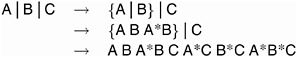
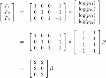
• When the response functions are the standard ones (generalized logits), then inclusion of the keyword _RESPONSE_ in every design effect induces a log-linear model. The design matrix for a log-linear model looks different from a standard design matrix because the standard one is transformed by the same linear transformation that converts the r response probabilities to r ˆ’ 1 generalized logits. For example, suppose the dependent variables X and Y each have two levels, and you specify a saturated log-linear model analysis:

    proc catmod;   model X*Y=_response_ / design;   loglin X Y X*Y;   run;  

• Then the cross-classification of X and Y yields four response probabilities, p ₁₁ , p ₁₂ , p ₂₁ , and p ₂₂ , which are then reduced to three generalized logit response functions, F ₁ = log( p ₁₁ /p ₂₂ ), F ₂ = log( p ₁₂ /p ₂₂ ),and F ₃ = log( p ₂₁ /p ₂₂ ).

• Since the saturated log-linear model implies that

  

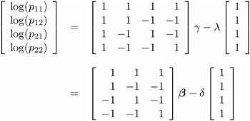
• where ³ and ² are parameter vectors, and » and are normalizing constants required by the restriction that the probabilities sum to 1, it follows that the MODEL statement yields

  

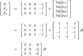
  Thus, the design matrix is as follows.

		Design Matrix
Sample	Number Response Function	X	Y	X*Y
1	1	2	2
1	2	2		ˆ’ 2
1	3		2	ˆ’ 2

Design matrices for reduced models are constructed similarly. For example, suppose you request a main-effects log-linear model analysis of the factors X and Y :

  proc catmod;   model X*Y=_response_ / design;   loglin X Y;   run;  

Since the main-effects log-linear model implies that

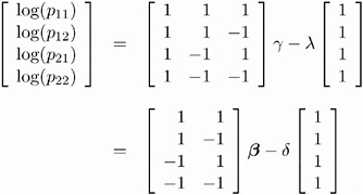
it follows that the MODEL statement yields

Therefore, the corresponding design matrix is as follows.

		Design Matrix
Sample	Response Function Number	X	Y
1	1	2	2
1	2	2
1	3		2

Since it is difficult to tell from the final design matrix whether PROC CATMOD used the parameterization that you intended, the procedure displays the untransformed _RESPONSE_ matrix for log-linear models. For example, the main-effects model in the preceding example induces the display of the following matrix.

Response Function Number	_Response_	Matrix
	1	2
1	1	1
2	1	ˆ’ 1
3	ˆ’ 1	1
4	ˆ’ 1	ˆ’ 1

You can suppress the display of this matrix by specifying the NORESPONSE option in the MODEL statement.

Cautions

Effective Sample Size

Since the method depends on asymptotic approximations, you need to be careful that the sample sizes are sufficiently large to support the asymptotic normal distributions of the response functions. A general guideline is that you would like to have an effective sample size of at least 25 to 30 for each response function that is being analyzed. For example, if you have one dependent variable and r = 4 response levels, and you use the standard response functions to compute three generalized logits for each population, then you would like the sample size of each population to be at least 75. Moreover, the subjects should be dispersed throughout the table so that less than 20 percent of the response functions have an effective sample size less than 5. For example, if each population had less than 5 subjects in the first response category, then it would be wiser to pool this category with another category rather than to assume the asymptotic normality of the first response function. Or, if the dependent variable is ordinally scaled, an alternative is to request the mean score response function rather than three generalized logits.

If there is more than one dependent variable, and you specify RESPONSE MEANS, then the effective sample size for each response function is the same as the actual sample size. Thus, a sample size of 30 could be sufficient to support four response functions, provided that the functions are the means of four dependent variables.

A Singular Covariance Matrix

If there is a singular (noninvertible) covariance matrix for the response functions in any population, then PROC CATMOD writes an error message and stops processing. You have several options available to correct this situation:

• You can reduce the number of response functions according to how many can be supported by the populations with the smallest sample sizes.

• If there are three or more levels for any independent variable, you can pool the levels into a fewer number of categories, thereby reducing the number of populations. However, your interpretation of results must be done more cautiously since such pooling implies a different sampling scheme and masks any differences that existed among the pooled categories.

• If there are two or more independent variables, you can delete at least one of them from the model. However, this is just another form of pooling, and the same cautions that apply to the previous option also apply here.

• If there is one independent variable, then, in some situations, you might simply eliminate the populations that are causing the covariance matrices to be singular.

• You can use the ADDCELL= option in the MODEL statement to add a small amount (for example, 0.5) to every cell frequency, but this can seriously bias the results if the cell frequencies are small.

Zero Frequencies

There are two types of zero cells in a contingency table: structural and sampling. A structural zero cell has an expected value of zero, while a sampling zero cell may have nonzero expected value and may be estimable .

If you use the standard response functions and there are zero frequencies, you should use maximum likelihood estimation (the default is ML=NR) rather than weighted least-squares to analyze the data. For weighted least-squares analysis, the CATMOD procedure always computes the observed response functions and may need to take the logarithm of a zero proportion. In this case, PROC CATMOD issues a warning and then takes the log of a small value (0 . 5 /n _i for the probability) in order to continue, but this can produce invalid results if the cells contain too few observations. Maximum likelihood analysis, on the other hand, does not require computation of the observed response functions and therefore yields valid results for the parameter estimates and all of the predicted values.

For a log-linear model analysis using WLS or ML=NR, PROC CATMOD creates response profiles only for the observed profiles. Thus, for any log-linear model analysis with one population (the usual case), the contingency table will not contain zeros, which means that all zero frequencies are treated as structural zeros. If there is more than one population, then a zero in the body of the contingency table is treated as a sampling zero (as long as some population has a nonzero count for that profile). If you fit the log-linear model using ML=IPF, the contingency table is incomplete and the zeros are treated like structural zeros. If you want zero frequencies that PROC CATMOD would normally treat as structural zeros to be interpreted as sampling zeros, you may specify the ZERO=SAMPLING and MISSING=SAMPLING options in the MODEL statement. Alternatively, you can specify ZERO=1E ˆ’ 20 and MISSING=1E ˆ’ 20.

Refer to Bishop, Fienberg, and Holland (1975) for a discussion of the issues and Example 22.5 on page 919 for an illustration of a log-linear model analysis of data that contain both structural and sampling zeros.

If you perform a weighted least-squares analysis on a contingency table that contains zero cell frequencies, then avoid using the LOG transformation as the first transformation on the observed proportions . In general, it may be better to change the response functions or to pool some of the response categories than to settle for the 0.5 correction or to use the ADDCELL= option.

Testing the Wrong Hypothesis

If you use the keyword _RESPONSE_ in the MODEL statement, and you specify MARGINALS, LOGITS, ALOGITS, or CLOGITS in your RESPONSE statement, you may receive the following warning message:

  Warning: The _RESPONSE_ effect may be testing the wrong   hypothesis since the marginal levels of the   dependent variables do not coincide. Consult the   response profiles and the CATMOD documentation.  

The following examples illustrate situations in which the _RESPONSE_ effect tests the wrong hypothesis.

Zeros in the Marginal Frequencies

Suppose you specify the following statements:

  data A1;   input Time1 Time2 @@;   datalines;   1 2    2 3    1 3   ;   proc catmod;   response marginals;   model Time1*Time2=_response_;   repeated Time 2 / _response_=Time;   run;  

One marginal probability is computed for each dependent variable, resulting in two response functions. The model is a saturated one: one degree of freedom for the intercept and one for the main effect of Time . Except for the warning message, PROC CATMOD produces an analysis with no apparent errors, but the 'Response Profiles' table displayed by PROC CATMOD is as follows.

Response Profiles
Response	Time1	Time2
1	1	2
2	1	3
3	2	3

Since RESPONSE MARGINALS yields marginal probabilities for every level but the last, the two response functions being analyzed are Prob(Time1=1) and Prob(Time2=2). Thus, the Time effect is testing the hypothesis that Prob(Time1=1)=Prob(Time2=2). What it should be testing is the hypothesis that

  Prob(Time1=1) = Prob(Time2=1)   Prob(Time1=2) = Prob(Time2=2)   Prob(Time1=3) = Prob(Time2=3)  

but there are not enough data to support the test (assuming that none of the probabilities are structural zeros by the design of the study).

The ORDER=DATA Option

Suppose you specify

  data a1;   input Time1 Time2 @@;   datalines;   2 1    2 2    1 1    1 2    2 1   ;   proc catmod order=data;   response marginals;   model Time1*Time2=_response_;   repeated Time 2 / _response_=Time;   run;  

As in the preceding example, one marginal probability is computed for each dependent variable, resulting in two response functions. The model is also the same: one degree of freedom for the intercept and one for the main effect of Time . PROC CATMOD issues the warning message and displays the following 'Response Profiles' table.

Response Profiles
Response	Time1	Time2
1	2	1
2	2	2
3	1	1
4	1	2

Although the marginal levels are the same for the two dependent variables, they are not in the same order because the ORDER=DATA option specified that they be ordered according to their appearance in the input stream. Since RESPONSE MARGINALS yields marginal probabilities for every level except the last, the two response functions being analyzed are Prob(Time1=2) and Prob(Time2=1). Thus, the Time effect is testing the hypothesis that Prob(Time1=2)=Prob(Time2=1). What it should be testing is the hypothesis that

  Prob(Time1=1) = Prob(Time2=1)   Prob(Time1=2) = Prob(Time2=2)  

Whenever the warning message appears, look at the 'Response Profiles' table or the 'One-Way Frequencies' table to determine what hypothesis is actually being tested . For the latter example, a correct analysis can be obtained by deleting the ORDER=DATA option or by reordering the data so that the (1,1) observation is first.

Computational Method

The notation used in PROC CATMOD differs slightly from that used in other literature. The following table provides a summary of the basic dimensions and the notation for a contingency table. See the 'Computational Formulas' section, which follows, for a complete description.

Summary of Basic Dimensions

s	=	number of populations or samples ( = number of rows in the underlying contingency table)
r	=	number of response categories (= number of columns in the underlying contingency table)
q	=	number of response functions computed for each population
d	=	number of parameters

Notation

j	denotes a column vector of 1s.
J	denotes a square matrix of 1s.
ˆ‘ k	is the sum over all the possible values of k .
n i	denotes the row sum ˆ‘ j n ij .
DIAG n ( p )	is the diagonal matrix formed from the first n elements of the vector p .
	is the inverse of DIAG n ( p ).
DIAG ( A 1 , A 2 , ..., A k )	denotes a block diagonal matrix with the A matrices on the main diagonal.

Input data can be represented by a contingency table, as shown in Table 22.4.

Table 22.4: Input Data Represented by a Contingency Table

	Response
Population	1	2		r	Total
1	n 11	n 12		n 1 r	n 1
2	n 21	n 22		n 2 r	n 2
s	n s 1	n s 2		n sr	n s

Computational Formulas

The following formulas are shown for each population and for all populations combined.

Source	Formula	Dimension
Probability Estimates
j th response		1 — 1
i th population		r — 1
all populations		sr — 1
Variance of Probability Estimates
i th population		r — r
all populations	V = DIAG ( V 1 , V 2 , , V s	sr — sr
Response Functions
i th population	F i = F ( p i )	q — 1
all populations		sq — 1
Derivative of Function with Respect to Probability Estimates
i th population		q — r
all populations	H = DIAG ( H 1 , H 2 , ..., H s )	sq — sr
Variance of Functions
i th population	S i = H i V i H i ²	q — q
all populations	S = DIAG ( S 1 , S 2 , ..., S s )	sq — sq
Inverse Variance of Functions
i th population	S i = ( S i ) ˆ’ 1	q — q
all populations	S ˆ’ 1 = DIAG ( S 1 , S 2 , ..., S s )	sq — sq

Derivative Table for Compound Functions: Y=F(G(p))

In the following table, let G ( p ) be a vector of functions of p , and let D denote ˆ‚ G / ˆ‚ p , which is the first derivative matrix of G with respect to p .

Function	Y = F ( G )	Derivative ( ˆ‚ Y / ˆ‚ p )
Multiply matrix	Y = A * G	A * D
Logarithm	Y = LOG ( G )	DIAG ˆ’ 1 ( G ) * D
Exponential	Y = EXP ( G )	DIAG ( Y ) * D
Add constant	Y = G + A	D

Default Response Functions: Generalized Logits

In the following table, subscripts i for the population are suppressed. Also denote for j = 1, ..., r ˆ’ 1 for each population i = 1 , ..., s .

Inverse of Response Functions for a Population

for j = 1, , r ˆ’ 1

Form of F and Derivative for a Population

F = KLOG(p) = (I _{r ˆ’ 1} , ˆ’ j) LOG(p)

Covariance Results for a Population

• where V , H , and J are as previously defined.

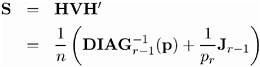
S ^{ˆ’ 1} = n(DIAG _{r ˆ’ 1} (p) ˆ’ qq ² ) where q = DIAG _{r ˆ’ 1} (p) j

The following calculations are shown for each population and then for all populations combined.

Source	Formula	Dimension
Design Matrix
i th population	X i	q — d
all populations		sq — d
Crossproduct of Design Matrix
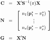
i th population	C i = X i ² S i X i	d — d
all populations	C = X ² S ˆ’ 1 X = ˆ‘ i C i	d — d

In the following table, z _p is the 100 p th percentile of the standard normal distribution.

Source	Formula	Dimension
Crossproduct of Design Matrix with Function
	R = X ² S ˆ’ 1 F = ˆ‘ i X i ² S i F i	d — 1
Weighted Least-Squares Estimates
	b = C ˆ’ 1 R = ( X ² S ˆ’ 1 X ) ˆ’ 1 ( X ² S ˆ’ 1 F )	d — 1
Covariance of Weighted Least-Squares Estimates
	COV ( b ) = C ˆ’ 1	d — d
Wald Confidence Limits for Parameter Estimates
		k = 1 , ..., d
Predicted Response Functions
		sq — 1
Covariance of Predicted Response Functions
		sq — sq
Residual Chi-Square
		1 — 1

Source	Formula	Dimension
Chi-Square for H : L ² =
	Q = ( Lb ) ² ( LC ˆ’ 1 L ² ) ˆ’ 1 ( Lb )	1 — 1

Maximum Likelihood Method

Let C be the Hessian matrix and G be the gradient of the log-likelihood function (both functions of and the parameters ² ). Let denote the vector containing the first r ˆ’ 1 sample proportions from population i , and let denote the corresponding vector of probability estimates from the current iteration. Starting with the least-squares estimates b of ² (if you use the ML and WLS options; with the ML option alone, the procedure starts with ), the probabilities ( b ) are computed, and b is calculated iteratively by the Newton-Raphson method until it converges (see the EPSILON= option on page 842). The factor » is a step-halving factor that equals one at the start of each iteration. For any iteration in which the likelihood decreases, PROC CATMOD uses a series of subiterations in which » is iteratively divided by two. The subiterations continue until the likelihood is greater than that of the previous iteration. If the likelihood has not reached that point after ten subiterations, then convergence is assumed, and a warning message is displayed.

Sometimes, infinite parameters may be present in the model, either because of the presence of one or more zero frequencies or because of a poorly specified model with collinearity among the estimates. If an estimate is tending toward infinity, then PROC CATMOD flags the parameter as infinite and holds the estimate fixed in subsequent iterations. PROC CATMOD regards a parameter to be infinite when two conditions apply:

• The absolute value of its estimate exceeds five divided by the range of the corresponding variable.

• The standard error of its estimate is at least three times greater than the estimate itself.

The estimator of the asymptotic covariance matrix of the maximum likelihood predicted probabilities is given by Imrey, Koch, and Stokes (1981, eq. 2.18).

The following equations summarize the method:

where

Iterative Proportional Fitting

The algorithm used by PROC CATMOD for iterative proportional fitting is described in Bishop, Fienberg, and Holland (1975), Haberman (1972), and Agresti (2002). To illustrate the method, consider the observed three-dimensional table { n _ijk } for the variables X, Y, and Z. The statements

  model X*Y*Z = _response_ / ml=ipf;   loglin XYZ@2;  

request that PROC CATMOD use IPF to fit the hierarchical model

Begin with a table of initial cell estimates PROC CATMOD produces the initial estimates by setting the n _sz structural zero cells to 0 and all other cells to n/ ( n _c ˆ’ n _sz ), where n is the total weight of the table and n _c is the total number of cells in the table. Iteratively adjust the estimates at step s ˆ’ 1 to the observed marginal tables specified in the model by cycling through the following three-stage process to produce the estimates at step s .

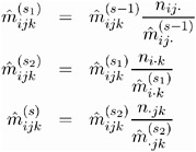
The subscript ' ·' indicates summation over the missing subscript. The log-likelihood l _s is estimated at each step s by

When the function ( l _{s ˆ’ 1} ˆ’ l _s ) /l _{s ˆ’ 1} is less than 10 ^{ˆ’ 8} , the iterations terminate. You can change the comparison value with the EPSILON= option, and you can change the convergence criterion with the CONV= option. The option CONV=CELL uses the maximum cell difference

as the criterion while the option CONV=MARGIN computes the maximum difference of the margins

Memory and Time Requirements

The memory and time required by PROC CATMOD are proportional to the number of parameters in the model.

Displayed Output

PROC CATMOD displays the following information in the 'Data Summary' table:

• the Response effect

• the Weight Variable, if one is specified

• the Data Set name

• the number of Response Levels

• the number of samples or Populations

• the Total Frequency, which is the total sample size

• the number of Observations from the data set (the number of data records)

• the frequency of missing observations, labeled as 'Frequency Missing'

Except for the analysis of variance table, all of the following items can be displayed or suppressed, depending on your specification of statements and options.

• The ONEWAY option produces the 'One-Way Frequencies' table, which displays the frequencies of each variable value used in the analysis.

• The populations (or samples) are defined in a table labeled 'Population Profiles.' The Sample Size and the values of the defining variables are displayed for each Sample. This table is suppressed if the NOPROFILE option is specified.

• The observed responses are defined in a table labeled 'Response Profiles.' The values of the defining variables are displayed for each Response. This table is suppressed if the NOPROFILE option is specified.

• If the FREQ option is specified, then the 'Response Frequencies' table is displayed, which shows the frequency of each response for each population.

• If the PROB option is specified, then the 'Response Probabilities' table is produced. This table displays the probability of each response for each population.

• If the COV option is specified, the 'Response Functions, Covariance Matrix' table, which shows the covariance matrix of the response functions for each Sample, is displayed.

• If the DESIGN option is specified, the Response Functions are displayed in the 'Response Functions, Design Matrix' table. If the COV option is also specified, the Response Functions are displayed in the 'Response Functions, Covariance Matrix' table.

• If the DESIGN option is specified, the design matrix is displayed in the 'Response Functions, Design Matrix' table, and if a log-linear model is being fit, the _RESPONSE_ matrix is displayed in the '_Response_ Matrix' table. If the model type is AVERAGED, then the design matrix is displayed with q * s rows, assuming q response functions for each of s populations. Otherwise, the design matrix is displayed with only s rows since the model is the same for each of the q response functions.

• The 'X ² *Inv(S)*X' matrix is displayed for weighted least-squares analyses if the XPX option is specified.

• The 'Analysis of Variance' table for the weighted least-squares analysis reports the results of significance tests for each of the design-effects in the righthand side of the MODEL statement. If _RESPONSE_ is a design-effect and is defined explicitly in the LOGLIN, FACTORS, or REPEATED statement, then the table contains test statistics for the individual effects constituting the _RESPONSE_ effect. If the design matrix is input directly, then the content of the displayed output depends on whether you specify any subsets of the parameters to be tested. If you specify one or more subsets, then the table contains one test for each subset. Otherwise, the table contains one test for the effect MODEL MEAN. In every case, the table also contains the Residual goodness-of-fit test. Produced for each test of significance are the Source of variation, the number of degrees of freedom (DF), the Chi-Square value (which is a Wald statistic), and the significance probability (Pr > ChiSq).

• The 'Analysis of Weighted Least-Squares Estimates' table lists, for each parameter in the model, the least-squares Estimate, the estimated Standard Error of the parameter estimate, the Chi-Square value (a Wald statistic, calculated as ((parameter estimate)/(standard error)) ² ) for testing that the parameter is zero, and the significance probability (Pr > ChiSq) of the test. If the CLPARM option is specified,then95% Wald confidence intervals are displayed.

  Each row in the table is labeled with the Parameter (the model effect and the class levels) and the response Function Number; however, if the NOPREDVAR option or a REPEATED or FACTORS statement is specified or if the design matrix is directly input, the rows are labeled by the Effect in the model for which parameters are formed and the Parameter number.

• The 'Covariance Matrix of the Parameter Estimates' table for the weighted least-squares analysis displays the estimated covariance matrix of the least-squares estimates of the parameters, provided the COVB option is specified.

• The 'Correlation Matrix of the Parameter Estimates' table for the weighted least-squares analysis displays the estimated correlation matrix of the least-squares estimates of the parameters, provided that the CORRB option is specified.

• The 'Maximum Likelihood Analysis' table is produced when the ML and ITPRINT options are specified for the standard response functions. It displays the Iteration number, the number of step-halving Sub-Iterations, ˆ’ 2 Log Likelihood for that iteration, the Convergence Criterion, and the Parameter Estimates for each iteration.

• The 'Maximum Likelihood Analysis of Variance' table, displayed when the ML option is specified for the standard response functions, is similar to the table produced for the least-squares analysis. The Chi-Square test for each effect is a Wald test based on the information matrix from the likelihood calculations. The Likelihood Ratio statistic compares the specified model with the unrestricted (saturated) model and is an appropriate goodness-of-fit test for the model.

• The 'Analysis of Maximum Likelihood Estimates' table, displayed when the ML option is specified for the standard response functions, is similar to the one produced for the least-squares analysis. The table includes the maximum likelihood estimates, the estimated Standard Errors based on the information matrix, and the Wald statistics (Chi-Square) based on estimated standard errors.

• The 'Covariance Matrix of the Maximum Likelihood Estimates' table displays the estimated covariance matrix of the maximum likelihood estimates of the parameters, provided that the COVB and ML options are specified for the standard response functions.

• The 'Correlation Matrix of the Maximum Likelihood Estimates' table displays the estimated correlation matrix of the maximum likelihood estimates of the parameters, provided that the CORRB and ML options are specified for the standard response functions.

• For each source of variation specified in a CONTRAST statement, the 'Contrasts' table lists the label for the source (Contrast), the number of degrees of freedom (DF), the Chi-Square value (which is a Wald statistic), and the significance probability (Pr > ChiSq). If the ESTIMATE= option is specified, the 'Analysis of Contrasts' table displays, for each row of the contrast, the label (Contrast), the Type (PARM or EXP), the Row of the contrast, the Estimate and its Standard Error, a Wald confidence interval, the Wald Chi-Square, and the p -value (Pr > ChiSq) for 1 degree of freedom.

• SpecificationofthePREDICT option in the MODEL statement has the following effect. Produced for each response function within each population are the Observed and Predicted Function values, their Standard Errors, and the Residual (Observed - Predicted). If the response functions are the default ones (generalized logits), additional information displayed for each response within each population includes the Observed and Predicted cell probabilities, their Standard Errors, and the Residual. However, specifying PRED=FREQ in the MODEL statement results in the display of the predicted cell frequencies, rather than the predicted cell probabilities. The displayed output includes the population profiles and, for the response function table, the Function Number, while the probability and frequency tables display the response profiles. If the NOPREDVAR option is specified in the MODEL statement, the population profiles are replaced with the Sample numbers, and the response profiles are replaced with the labels P n for the n th cell probability, and F n for the n th cell frequency.

• When there are multiple RESPONSE statements, the output for each statement starts on a new page. For each RESPONSE statement, the corresponding title, if specified, is displayed at the top of each page.

• If the ADDCELL= option is specified in the MODEL statement, and if there is a weighted least-squares analysis specified, the adjusted sample size for each population (with number added to each cell) is labeled Adjusted Sample Size in the 'Population Profiles' table. Similarly, the adjusted response frequencies and probabilities are displayed in the 'Adjusted Response Frequencies' and 'Adjusted Response Probabilities' tables, respectively.

• If _RESPONSE_ is defined explicitly in the LOGLIN, FACTORS, or REPEATED statement, then the definition is displayed as a NOTE whenever _RESPONSE_ appears in the output.

ODS Table Names

PROC CATMOD assigns a name to each table it creates. You can use these names to reference the table when using the Output Delivery System (ODS) to select tables and create output data sets. These names are listed in the following table. For more information on ODS, see Chapter 14, 'Using the Output Delivery System.'

Table 22.5: ODS Tables Produced in PROC CATMOD

ODS Table Name	Description	Statement	Option
ANOVA	Analysis of variance	MODEL	default
Contrasts	Contrasts	CONTRAST	default
ContrastEstimates	Analysis of Contrasts	CONTRAST	ESTIMATE=
ConvergenceStatus	Convergence status	MODEL	ML
CorrB	Correlation matrix of the estimates	MODEL	CORRB
CovB	Covariance matrix of the estimates	MODEL	COVB
DataSummary	Data summary	PROC	default
Estimates	Analysis of estimates	MODEL	default, unless NOPARM
MaxLikelihood	Maximum likelihood analysis	MODEL	ML and ITPRINT
OneWayFreqs	One-way frequencies	MODEL	ONEWAY
PopProfiles	Population profiles	MODEL	default, unless NOPROFILE
PredictedFreqs	Predicted frequencies	MODEL	PRED=FREQ
PredictedProbs	Predicted probabilities	MODEL	PREDICT or PRED=PROB
PredictedValues	Predicted values	MODEL	PREDICT or PRED=
ResponseCov	Response functions, covariance matrix	MODEL	COV
ResponseDesign	Response functions, design matrix	MODEL	DESIGN, unless NODESIGN
ResponseFreqs	Response frequencies	MODEL	FREQ
ResponseMatrix	_RESPONSE_ matrix	MODEL & LOGLIN	DESIGN, unless NORESPONSE
ResponseProbs	Response probabilities	MODEL	PROB
ResponseProfiles	Response profiles	MODEL	default, unless NOPROFILE
XPX	X '*Inv( S )* X matrix	MODEL	XPX, for WLS [*]
[*] WLS estimation is the default for response functions other than the default (generalized logits).