Chapter Five: Working with Worksheet and Workbooks

Lesson 1: Working with Rows and Columns

Inserting Rows and Columns

Inserting rows and columns is necessary if you have to enter a series of text in a table and there are no enough rows and columns for it.

To insert rows or columns, follow these steps:

Do one of the following:

Insert a single row.	Click a cell in the row immediately below where you want the new row.
Example: To insert a new row above row 5, click the row heading number 5, and then right-click and choose Insert.
Insert multiple rows.	Select rows immediately below where you want the new rows. Select the same number of rows as you want to insert.
Insert a single column.	Click a cell in the column immediately to the right of where you want to insert the new column.
Example: To insert a new column to the left of column B, click a cell in column B.
Insert multiple columns.	Select columns immediately to the right of where you want to insert the new columns. Select the same number of columns you want to insert.

Do one of the following:
- On the Insert menu, click Rows, or Columns.
- Right-click the row heading and choose Insert.

Deleting Rows or Columns

Deleting rows or columns removes them from the worksheet and move the cells to fill the space where they were.

To delete rows or columns, follow these steps:

Select the row or column headings you want to delete.
Do one of the following:
- Right-click row or column heading and choose Delete.
- Click the Edit menu and choose Delete.

Hiding Rows or Columns

Hiding rows and columns helps you organize a large worksheet.

Hide rows or columns

Select the row or column heading you want to hide.
Do one of the following:
- Click the Format menu, choose Row or Column, and then choose Hide.
- Right-click the row or column, then click Hide.
- Press Ctrl+9 to hide rows or Ctrl+0 to hide columns.

Unhide rows or columns

To display hidden rows or columns, do any of the following:
- Select the row heading number above and below the hidden area to unhide rows.
- Select the column heading letters to the left and right of the hidden area to unhide columns.
- Click the Select All button or press Ctrl+A to unhide all rows and columns.
Do one of the following:
- Click the Format menu, choose Row or Column, and then click Unhide.
- Press Ctrl+Shift+( (open parenthesis) to unhide rows or Ctrl+Shift+) (close parenthesis) to unhide columns.
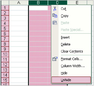
- Right-click the row or column headings, and choose Unhide.

Freeze and Unfreeze Rows and Columns

One way of viewing the parts of your worksheet while working on a large worksheet is by using the option to freeze rows and columns. In the Window menu, you have an option to immobilize your rows and columns using the Freeze Panes option. Freezing panes will either lock the top and/or upper-left panes depending on where you have placed your pointer.

To freeze panes, follow the steps below:

Move the cell pointer below any rows and to the right of any columns you want to freeze.
Click the Window menu and choose Freeze Panes.

To unfreeze rows and columns, click the Windows menu and choose Unfreeze Panes.

Splitting Worksheet

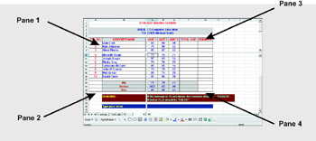
Freezing rows and columns allows you to view some parts of the worksheet. Another way to make it easier for you to view some portions of the worksheet is to split it. This will enable you to view different sections of the worksheet side by side in separate panes. Panes are the sections of the worksheet.

An alternative to freezing the rows or columns is to split the worksheet. A split worksheet enables you to view different sections of the worksheet side-by-side in separate panes. Each section of a worksheet is referred to as a pane.

To split the worksheet, do the following:

Move the cell pointer below any rows and to the right of any columns where you want the split to occur.
Click the Window menu and choose Split.
Click the mouse pointer in one of the panes and use the scroll bars to move to that pane.

To remove a split window:
- Click Window from the menu bar, then choose Remove Split.
- Press Alt+W and then press S.

Note

To adjust or remove panes, you simply rest your pointer to the split bar until it becomes a double arrow. Drag it to a new location or to row or column heading.

Whiz Words

Panes	Freeze Panes
Column	Row
Split

Lesson Summary

Inserting and deleting rows and columns helps you add space for or get rid of extra data. Select one or more rows or columns, right-click a row or column header, and choose Insert or Delete.

Hiding rows and columns helps you organize a large worksheet.

Excel allows you to view multiple panes in your worksheet. You can also freeze and unfreeze a portion of your worksheet. To split a window, move the active cell where you want the worksheet to split, and then choose the Split option in the Window menu.

Study Help

What is a pane? When are we going to freeze panes?
What keys should we press to remove the split of a Worksheet?
How to add rows and columns? Give two ways to add rows and columns.

Activity 1

Open the file Sum Function.xls.
Hide the column that contains the Total Quizzes.
Delete columns 18, 19 and 20.
Make cell C6 the active cell.
Click Freeze Panes in the Windows menu.
Save your work as Freeze.xls at Excel-Activities folder.