Chapter 14: Limited Mathematical Background for Design for Six Sigma (DFSS)

EXPONENTIAL DISTRIBUTION AND RELIABILITY

EXPONENTIAL DISTRIBUTION

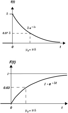
Probability Density Function and Cumulative Distribution Function

Probability Density Function (Decay Time)

Cumulative Distribution Function (Rise Time)

F(t) ‰ e ^{- t} dt = 1 - e ^{- t}

Mean Time:

Variance:

One parameter:

Reliability Problems

Exponential distribution is used in reliability problems.

Exponential distribution can describe the probability of a failure prior to some specified time t assuming that failure occurs at a constant rate ( = » ) over time.

Reliability, the chance of no failure in time t, is expressed as

R ( t ) = e ^{- t}

Failure is a complement of cumulative probability of reliability:

F ( t ) ‰ 1 - R ( t ) = 1 - e ^{- t}

F(t) is used to compute the probability of failure prior to t.

The derivative of the cumulative distribution function is the probability density function (pdf).

Mean Time to Failure (MTTF) = T _MF =

Failure Rate: = 1/ T _MF

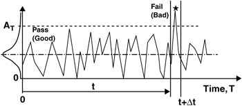
CONSTANT RATE FAILURE

Exponential function: Ae ^{- t}

Evaluate at any time t, the time rate of decrease in amplitude is constant:

If we consider equal time increments At, then exponential has consistent amplitude ratio between increments

Example

Data from 100 pumps demonstrated an average life of 5.75 years and that failures followed an exponential distribution.

Problems and Solutions:

1.	Determine the probability of failure during the first year.
2.	Determine the probability of failure during the first 3 months.
3.	Determine the probability of failure prior to the average life.
4.	Determine the probability of reliably operating for at least 10 years.
5.	Plot the reliability curve and compare with the pdf curve. Given: MTTF = T MF = 1/ = 5.75 years Compute Failure Rate: = 1/T MF = 0.174 per year Exponential pdf: f ( t ) = e - t = 0.174 e -0.174 t Failure cdf: F ( t ) = 1 - R ( t ) = 1 - e - t

Answers

1.	Probability of failure during the first year: 16%
2.	Probability of failure during the first 3 months or 1/4 year:
3.	Probability of failure prior to the average life; MTTF = T MF = 5.75
4.	Probability of reliably operating for at least 10 years.
5.	Plot the reliability curve and compare with the pdf curve.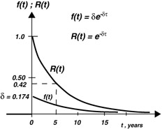

PROBABILITY OF RELIABILITY

The exponential distribution as the basis of the reliability function is based on the probability of samples of an event that describes a general physical situation; i.e., time to a (bad) occurrence.

CONTROL CHARTS

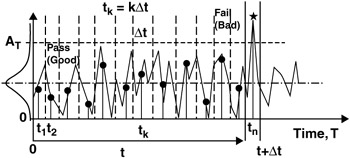
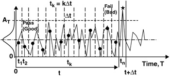
Continuous Time Waveform

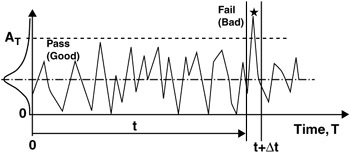
Discrete Time Samples

Digital Signal Processing

• Uniform sampling time or time increment: t _s = ” t

• Time increment ” t small so as to include only one sample.

• Total sampling time: t _n = nt _s = n ˆ t

• Total number of samples taken: n = t _n / t _s

• Current time sample: t _k = kt _s = k ˆ t

• Designate RV event as occurrence of bad sample X.

• Probability of a bad sample only in the n-th interval.

SAMPLE SPACE

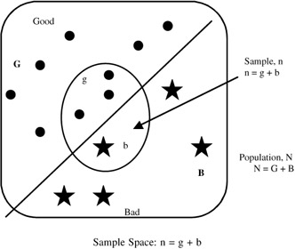
• Sample "Bad" when outcome exceeds a limit A _T

• Sample "Good" when outcome less than limit A _T

• Random variable for this experiment is X.

• "Good" or "Bad" are the only two possible states for X.

• Assign

• X = 0 for "Good"

• X = 1 for "Bad"

Sample Space: n = g + b

One bad sample {b} is assumed to occur exactly on the n-sample.

{b} = {X _n = 1}

This single bad sample is preceded by a sequence of (n - 1) good samples {g}.

{g} = {X _{n - 1} = 0, X _{n - 2} = 0, ..., X ₁ = 0}

If each sample is independent of the proceeding sample then

ASSIGNING PROBABILITY TO SETS

Assume only one sample can be measured in any interval ” t.

• The probability that one bad sample occurs in interval is assumed to be constant

  p = ” t

  

• Conversely, the probability of one good sample in this interval is

  

• The probability of (n - 1) good samples in the range [0 ‰ T ‰ t] is

  

• Probability of total set:

  

Note  

There are two types of probabilities or variables , one when X = 0 for set {g} and one when X = 1 for set {b}.

To establish an "equation," we need to deal with only one variable.

Assume the sample of the increment where also "good" then we could write directly:

Differential equation form (take limit as ” t ’ dt):

Dividing by dt puts the LHS into the form of a derivative:

First order differential equation (homogeneous):

which can be conveniently expressed in terms of reliability:

• Solution: R = e ^{- t} + C ₁

• Initial condition at t = 0: R = 1 = 1 + C ₁ and C ₁ = 0

• Hence, the reliability is: R = e ^{- t} ₁