Details

Statistical Tests

The following section discusses the statistical tests performed in the MULTTEST procedure. For continuous data, a t -test for the mean is available. For discrete variables , available tests are the Cochran-Armitage (CA) linear trend test, the Freeman-Tukey (FT) double arcsine test, the Peto mortality-prevalence test, and the Fisher exact test.

Throughout this section, the discrete and continuous variables are denoted by S _vgsr and X _vgsr , respectively, where v is the variable, g is the treatment group , s is the stratum, and r is the replication. A plus sign (+) subscript denotes summation over an index. Note that the tests are invariant to the location and scale of the contrast coefficients t _g .

Cochran-Armitage Linear Trend Test

The Cochran-Armitage linear trend test (Cochran 1954; Armitage 1955; Agresti 1990) is implemented using a Z -score approximation , an exact permutation distribution, or a combination of both.

Z-Score Approximation

Let m _vgs denote the sample size for a binary variable v within group g and stratum s . The pooled probability estimate for variable v and stratum s is

The expected value (under constant within-stratum treatment probabilities) for variable v , group g , and stratum s is

The test statistic for variable v has numerator

where t _g denotes the contrast trend coefficients specified by the CONTRAST statement. The binomial variance estimate for this statistic is

where

The hypergeometric variance estimate (the default) is

For any strata s with m _{v + s} ‰ 1, the contribution to the variance is taken to be zero.

PROC MULTTEST computes the Z -score statistic

The p -value for this statistic comes from the standard normal distribution. Whenever a 0 is computed for the denominator, the p -value is set to 1. This p -value approximates the probability obtained from the exact permutation distribution, discussed in the following text.

The Z -score statistic can be continuity-corrected to better approximate the permutation distribution. With continuity correction c , the upper-tailed p -value is computed from

For two-tailed, noncontinuity-corrected tests, PROC MULTTEST reports the p -value as 2min( p, 1 ˆ’ p ), where p is the upper-tailed p -value. The same formula holds for the continuity-corrected test, with the exception that when the noncontinuity-corrected Z and the continuity-corrected Z have opposite signs, the two-tailed p -value is 1.

When the PERMUTATION= option is specified and no STRATA variable is specified, PROC MULTTEST uses a continuity correction selected to optimally approximate the upper-tail probability of permutation distributions with smaller marginal totals (Westfall and Lin 1988). Otherwise, the continuity correction is specified using the CONTINUITY= option in the TEST statement.

The CA Z -score statistic is the Hoel-Walburg (Mantel-Haenszel) statistic reported by Dinse (1985).

Exact Permutation Test

When you use the PERMUTATION= option for CA in the TEST statement, PROC MULTTEST computes the exact permutation distribution of the trend score

and then compares the observed value of this trend with the permutation distribution to obtain the p -value

where X is a random variable from the permutation distribution and where uppertailed tests are requested . This probability can be viewed as a binomial probability, where the within-stratum probabilities are constant and where the probability is conditional with respect to the marginal totals S _{v + s +} . It also can be considered a rerandomization probability.

Because the computations can be quite time-consuming with large data sets, specifying the PERMUTATION= number option in the TEST statement limits the situations where PROC MULTTEST computes the exact permutation distribution. When marginal total success or total failure frequencies exceed number for a particular stratum, the permutation distribution is approximated using a continuity-corrected normal distribution. You should be cautious in using the PERMUTATION= option in conjunction with bootstrap resampling because the permutation distribution is recomputed for each bootstrap sample. This recomputation is not necessary with permutation resampling.

The permutation distribution is computed in two steps:

1. The permutation distributions of the trend scores are computed within each stratum.

2. The distributions are convolved to obtain the distribution of the total trend.

As long as the total success or failure frequency does not exceed number for any stratum, the computed distributions are exact. In other words, if S _{v + s +} ‰ number or ( m _{v + s} ˆ’ S _{v + s +} ) ‰ number for all s , then the permutation trend distribution for variable v is computed exactly.

In step 1, the distribution of the within-stratum trend

is computed using the multivariate hypergeometric distribution of the S _{vgs +} , provided number is not exceeded. This distribution can be written as

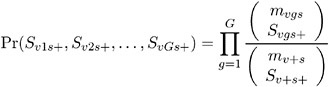
The distribution of the within-stratum trend is then computed by summing these probabilities over appropriate configurations. For further information on this technique, refer to Bickis and Krewski (1986) and Westfall and Lin (1988). In step 2, the exact convolution distribution is obtained for the trend statistic summed over all strata having totals that meet the threshold criterion. This distribution is obtained by applying the fast Fourier transform to the exact within-stratum distributions. A description of this general method can be found in Pagano and Tritchler (1983) and Good (1987).

The convolution distribution of the overall trend is then computed by convolving the exact distribution with the distribution of the continuity-corrected standard normal approximation. To be more specific, let S ₁ denote the subset of stratum indices that satisfy the threshold criterion, and let S ₂ denote the subset of indices that do not satisfy the criterion. Let T _{v 1} denote the combined trend statistic from the set S ₁ , which has an exact distribution obtained using Fourier analysis as previously outlined, and let T _{v 1} denote the combined trend statistic from the set S ₂ . Then the distribution of the overall trend T _v = T _{v 1} + T _{v 2} is obtained by convolving the analytic distribution of T _{v 1} with the continuity-corrected normal approximation for T _{v 2} . Using the notation from the Z-Score Approximation section on page 2948, this convolution can be written as

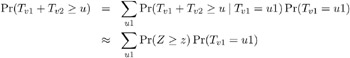
where Z is a standard normal random variable, and

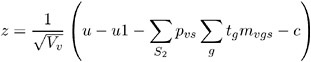
In this expression, the summation of s in V _v is over S ₂ , and c is the continuity correction discussed under the Z -score approximation.

When a two-tailed test is requested, the expected trend

is computed, and the two-tailed p -value is reported as the permutation tail probability for the observed trend T _v plus the permutation tail probability for 2 E _v ˆ’ T _v , the reflected trend.

Freeman-Tukey Double Arcsine Test

For this test, the contrast trend coefficients t ₁ ,...,t _G are centered to the values c ₁ ,..., c _G , where c _g = t _g ˆ’ t , t = ˆ‘ _g t _g /G , and G is the number of groups. The numerator of this test statistic is

where the weights w _vs take on three different types of values depending upon your specification of the WEIGHT= option in the STRATA statement. The default value is the within-strata sample size m _{v + s} , ensuring comparability with the ordinary CA trend statistic. WEIGHT= HARMONIC sets w _vs equal to the harmonic mean

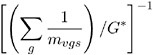
where G * is the number of non-missing groups and the summation is over only the non-missing elements. The harmonic means analysis places more weight on the smaller sample sizes than does the default sample size method, and is similar to a Type 2 analysis in PROC GLM. WEIGHT=EQUAL sets w _vs = 1 for all v and s , and is similar to a Type 3 analysis in PROC GLM.

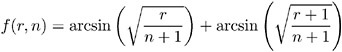
The function f ( r, n ) is the double arcsine transformation:

The variance estimate is

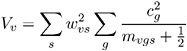
and the test statistic is

The Freeman-Tukey transformation and its variance are described by Freeman and Tukey (1950) and Miller (1978). Since its variance is not weighted by the pooled probabilities, as is the CA test, the FT test can be more useful than the CA test for tests involving only a subset of the groups.

Peto Mortality-Prevalence Trend Test

The Peto test is a modified Cochran-Armitage procedure incorporating mortality and prevalence information. It represents a special case in PROC MULTTEST because the data structure requirements are different, and the resampling methods used for adjusting p -values are not valid. The TIME= option variable is required to specify death times or, more generally , time of occurrence. In addition, the test variables must assume one of the following three values.

• 0 = no occurrence

• 1 = incidental occurrence

• 2 = fatal occurrence

Use the TIME= option variable to define the mortality strata, and use the STRATA statement variable to define the prevalence strata.

The Peto test is computed like two Cochran-Armitage Z -score approximations, one for prevalence and one for mortality.

In the following notation, the subscript v represents the variable, g represents the treatment group, s represents the stratum, and t represents the time. Recall that a plus sign (+) in a subscript location denotes summation over that subscript.

Let be the number of incidental occurrences, and let be the total sample size for variable v in group g , stratum s , excluding fatal tumors .

Let be the number of fatal occurrences in time period t , and let be the number alive at the end of time t ˆ’ 1.

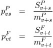
The pooled probability estimates are

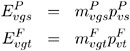
The expected values are

Define the numerator terms:

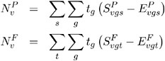
where t _g denotes a contrast trend coefficient. Define the denominator variance terms (using the binomial variance):

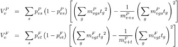
The hypergeometric variances (the default) are calculated by weighting the within-strata variances as discussed in the Z-Score Approximation section on page 2948.

The Peto statistic is computed as

where c is a continuity correction. The p -value is determined from the standard normal distribution unless the PERMUTATION= number option is used. When you use the PERMUTATION= option for PETO in the TEST statement, PROC MULTTEST computes the discrete approximation permutation distribution described by Mantel (1980) and Soper and Tonkonoh (1993). Specifically , the permutation distribution of

is computed, assuming that and are independent over all s and t . The p -values are exact under this independence assumption. However, the independence assumption is valid only asymptotically, which is why these p -values are called approximate.

An exact permutation distribution is available only under the assumption of equal risk of censoring in all treatment groups; even then, computing this distribution can be cumbersome. Soper and Tonkonoh (1993) describe situations where the discrete approximation distribution closely fits the exact permutation distribution.

Fisher Exact Test

The CONTRAST statement in PROC MULTTEST enables you to compute Fisher exact tests for two-group comparisons. No stratification variable is allowed for this test. Note, however, that the FISHER exact test is a special case of the exact permutation tests performed by PROC MULTTEST and that these permutation tests allow astratification variable. Recall that contrast coefficients can be ˆ’ 1, 0, or 1 for the Fisher test. The frequencies and sample sizes of the groups scored as ˆ’ 1 are combined, as are the frequencies and sample sizes of the groups scored as 1. Groups scored as 0 are excluded. The ˆ’ 1 group is then compared with the 1 group using the Fisher exact test.

Letting x and m denote the frequency and sample size of the 1 group, and y and n denote those of the ˆ’ 1 group, the p -value is calculated as

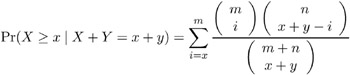
where X and Y are independent binomially distributed random variables with sample sizes m and n and common probability parameters. The hypergeometric distribution is used to determine the stated probability; Yates (1984) discusses this technique. PROC MULTTEST computes the two-tailed p -values by adding probabilities from both tails of the hypergeometric distribution. The first tail is from the observed x and y , and the other tail is chosen so that the resulting probability is as large as possible without exceeding the probability from the first tail.

t-Test for the Mean

For continuous variables, PROC MULTTEST automatically centers the contrast trend coefficients, as in the Freeman-Tukey test. These centered coefficients c _g are then used to form a t -statistic contrasting the within-group means. Let n _vgs denote the sample size within group g and stratum s ; it depends on variable v only when there are missing values. Define

as the sample mean within a group-and-stratum combination, and define

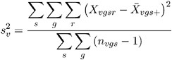
as the pooled sample variance. Assume constant variance for all group-and-stratum combinations. Then the t -statistic for the mean is

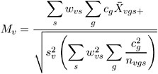
where the weights w _vs are determined as in the Freeman-Tukey test with n _vgs replacing m _vgs .

Let ¼ _vgs denote the treatment means. Then under the null hypothesis that

and assuming normality, independence, and homoscedasticity, M _v follows a t -distribution with ˆ‘ _s ˆ‘ _g ( n _vgs ˆ’ 1) degrees of freedom.

Whenever a denominator of 0 is computed, the p -value is set to 1. When missing data force n _vgs = 0, then the contribution to the denominator of the pooled variance is 0 and not ˆ’ 1. This is also true for degrees of freedom.

p-Value Adjustments

PROC MULTTEST offers p -value adjustments using Bonferroni, Sidak, Bootstrap resampling, and Permutation resampling, all with single-step or stepdown versions. In addition, Hochberg s (1988) and Benjamini and Hochberg s (1995) step-up methods are offered , as are Hommel s (1988) and Fisher s combination method. The Bonferroni and Sidak methods are calculated from the permutation distributions when exact permutation tests are used with CA or PETO tests.

All methods but the resampling methods are calculated using simple functions of the raw p -values or marginal permutation distributions; the permutation and bootstrap adjustments require the raw data. Because the resampling techniques incorporate distributional and correlational structures, they tend to be less conservative than the other methods.

When a resampling (bootstrap or permutation) method is used with only one test, the adjusted p -value is the bootstrap or permutation p -value for that test, with no adjustment for multiplicity, as described by Westfall and Soper (1994).

Bonferroni

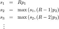
Suppose that PROC MULTTEST performs R statistical tests, yielding p -values p ₁ ,...,p _R . Then the Bonferroni p -value for test r is simply Rp _r . If the adjusted p -value exceeds 1, it is set to 1.

If the unadjusted p -values are computed using exact permutation distributions, then the Bonferroni adjustment for p _r is , where is the largest p -value from the permutation distribution of test j satisfying , or 0 if all permutational p -values of test j are greater than p _r . These adjustments are much less conservative than the ordinary Bonferroni adjustments because they incorporate the discrete distributional characteristics. However, they remain conservative in that they do not incorporate correlation structures between multiple contrasts and multiple variables (Westfall and Wolfinger 1997).

Sidak

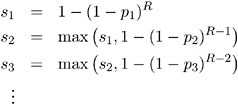
A technique slightly less conservative than Bonferroni is the Sidak p -value (Sidak 1967), which is 1 ˆ’ (1 ˆ’ p _r ) ^R . It is exact when all of the p -values are uniformly distributed and independent, and it is conservative when the test statistics satisfy the positive orthant dependence condition (Holland and Copenhaver 1987).

If the unadjusted p -values are computed using exact permutation distributions, then the Sidak adjustment for p _r is , where the are as described previously. These adjustments are less conservative than the corresponding Bonferroni adjustments, but they do not incorporate correlation structures between multiple contrasts and multiple variables (Westfall and Wolfinger 1997).

Bootstrap

The bootstrap method creates pseudo-data sets by sampling observations with replacement from each within-stratum pool of observations. An entire data set is thus created, and p -values for all tests are computed on this pseudo-data set. A counter records whether the minimum p -value from the pseudo-data set is less than or equal to the actual p -value for each base test. (If there are R tests, then there are R such counters.) This process is repeated a large number of times, and the proportion of resampled data sets where the minimum pseudo- p -value is less than or equal to an actual p -value is the adjusted p -value reported by PROC MULTTEST. The algorithms are described by Westfall and Young (1993).

In the case of continuous data, the pooling of the groups is not likely to recreate the shape of the null hypothesis distribution, since the pooled data are likely to be multimodal. For this reason, PROC MULTTEST automatically mean-centers all continuous variables prior to resampling. Such mean-centering is akin to resampling residuals in a regression analysis, as discussed by Freedman (1981). You can specify the NOCENTER option if you do not want to center the data. (In most situations, it does not seem to make much difference whether or not you center the data.)

The bootstrap method explicitly incorporates all sources of correlation, from both the multiple contrasts and the multivariate structure. The adjusted p -values incorporate all correlations and distributional characteristics.

Permutation

The permutation-style adjusted p -values are computed in identical fashion as the bootstrap adjusted p -values, with the exception that the within-stratum resampling is performed without replacement instead of with replacement. This produces a rerandomization analysis such as in Brown and Fears (1981) and Heyse and Rom (1988). In the spirit of rerandomization analyses, the continuous variables are not centered prior to resampling. This default can be overridden by using the CENTER option.

The permutation method explicitly incorporates all sources of correlation, from both the multiple contrasts and the multivariate structure. The adjusted p -values incorporate all correlations and distributional characteristics.

Stepdown Methods

Stepdown testing is available for the Bonferroni, Sidak, bootstrap, and permutation methods. The benefit of using stepdown methods is that the tests are made more powerful (smaller adjusted p -values) while, in most cases, maintaining strong control of the familywise error rate. The stepdown method was pioneered by Holm (1979) and further developed by Shaffer (1986), Holland and Copenhaver (1987), and Hochberg and Tamhane (1987).

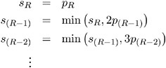
Suppose the base test p -values are ordered as p ₁ < p ₂ < · · · < p _R . The Bonferroni stepdown p -values s ₁ ,...,s _R are obtained from

As always, if any adjusted p -value exceeds 1, it is set to 1. The Sidak stepdown p -values are determined similarly:

Stepdown Bonferroni adjustments using exact tests are defined as

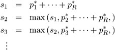
where the are defined as before. Note that is taken from the permutation distribution corresponding to the j th smallest unadjusted p -value. Also, any s _j greater than 1.0 is truncated to 1.0.

Stepdown Sidak adjustments for exact tests are defined analogously by substituting

The resampling-style stepdown method is analogous to the preceding stepdown methods; the most extreme p -value is adjusted according to all R tests, the second-most extreme p -value is adjusted according to ( R ˆ’ 1) tests, and so on. The difference is that all correlational and distributional characteristics are incorporated when you use resampling methods. More specifically, assuming the same ordering of p -values as discussed previously, the resampling-style stepdown adjusted p -value for test r is the probability that the minimum pseudo- p -value of tests r,...,R is less than or equal to p _r .

This probability is evaluated using Monte Carlo, as are the previously described resampling-style adjusted p -values. In fact, the computations for stepdown adjusted p -values are essentially no more time-consuming than the computations for the non-stepdown adjusted p -values. After Monte Carlo, the stepdown adjusted p -values are corrected to ensure monotonicity; this correction leaves the first adjusted p -values alone, then corrects the remaining ones as needed. The stepdown method approximately controls the familywise error rate, and it is described in more detail by Westfall and Young (1993), Westfall et al. (1999), and Westfall and Wolfinger (2000).

Hochberg

Assuming p -values are independent and uniformly distributed under their respective null hypotheses, Hochberg (1988) demonstrated that Holm s stepdown adjustments control the familywise error rate even when calculated in step-up fashion. Since the adjusted p -values are uniformly smaller for Hochberg s method than for Holm s method, the Hochberg method is more powerful. However, this improved power comes at the cost of having to make the assumption of independence.

The Hochberg adjusted p -values are defined in reverse order as the stepdown Bonferroni:

Hommel

Hommel s (1988) method is a closed testing procedure based on Simes (1986) test. The Simes p -value for a joint test of any set of S hypotheses with p -values p ₁ ‰ p 2 ‰ ... ‰ p _S is min(( S/ 1) p ₁ , ( S/ 2) p ₂ ,..., ( S/S ) p _S ). The Hommel adjusted p -value for test j is the maximum of all such Simes p -values, taken over all joint tests that include j as one of their components .

Hochberg adjusted p -values are always as large or larger than Hommel adjusted p -values. Sarker and Chang (1997) showed that Simes method is valid under independent or positively dependent p -values, so Hommel s and Hochberg s methods also are valid in such cases by the closure principle.

Fisher Combination

The FISHER_C option requests adjusted p -values using closed tests, based on the idea of Fisher s combination test. The Fisher combination test for a joint test of any set of S hypotheses with p -values uses the chi-square statistic ² = ˆ’ 2 ˆ‘ log( p _i ), with 2 S degrees of freedom. The FISHER_C adjusted p -value for test j is the maximum of all p -values for the combination tests, taken over all joint tests that include j as one of their components. Independence of p -values is required for the validity of this method.

False Discovery Rate

The FDR option requests p -values that control the false discovery rate, described by Benjamini and Hochberg (1995). These adjustments are potentially much less conservative than the Hochberg adjustments; however, they do not necessarily control the familywise error rate. Furthermore, they are guaranteed to control the false discovery rate only with independent p -values that are uniformly distributed under their respective null hypotheses.

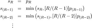
The FDR adjusted p -values are defined in step-up fashion, like the Hochberg adjustments, but with less conservative multipliers:

Missing Values

If a CLASS or STRATA variable has a missing value, then PROC MULTTEST removes that observation from the analysis.

When there are missing values for test variables, the within group-and-stratum sample sizes may differ from variable to variable. In most cases this is not a problem; however, it is possible for all data to be missing for a particular group within a particular stratum. For continuous variables and Freeman-Tukey tests, PROC MULTTEST recenters the contrast trend coefficients within strata where all data for a particular group are missing. The Cochran-Armitage and Peto tests are unaffected by this situation.

PROC MULTTEST uses missing values for resampling if they exist in the original data set. If all variables have missing values for any observation, then PROC MULTTEST removes it prior to resampling. Otherwise, PROC MULTTEST treats all missing values as ordinary observations in the resampling. This means that different resampled data sets can have different group sizes. In some cases it means that a resampled data set can have all missing values for a particular variable in a particular group/stratum combination, even when values exist for that combination in the original data. For this reason, PROC MULTTEST recomputes all quantities within each pseudo-data set, including such items as centered scoring coefficients and degrees of freedom for p -values.

While PROC MULTTEST does provide analyses in missing value cases, you should not feel that it completely solves the missing value problem. If you are concerned about the adverse effects of missing data on a particular analysis, you should consider using imputation and sensitivity analyses to assess the effects of the missing data.

Computational Resources

PROC MULTTEST keeps all of the data in memory to expedite resampling. A large portion of the memory requirement is thus 8*NOBS*NVAR bytes, where NOBS is the number of observations in the data set, and NVAR is the number of variables analyzed , including CLASS, FREQ, and STRATA variables.

If you specify PERMUTATION= number (for exact permutation distributions), then PROC MULTTEST requires additional memory. This requirement is approximately 4*NTEST*NSTRATA*CMAX* number *( number +1) bytes, where NTEST is the number of contrasts, NSTRATA is the number of STRATA levels, and CMAX is the maximum contrast coefficient.

The execution time is linear in the number of resamples; that is, 10,000 resamples will take 10 times longer than 1,000 resamples.

Output Data Sets

OUT= Data Set

The OUT= data set contains contrast names ( _test_ ), variable names ( _var_ ), the contrast label ( _contrast_ ), raw p -values ( raw_p ), and all requested adjusted p -values ( bon_p , sid_p , stpbon_p , stpsid_p , boot_p , perm_p , stpbootp , stp- permp , hoc_p , or fdr_p ).

If a resampling-based adjusted p -value is requested, then the simulation standard error is included as either sim_se or stpsimse , depending upon whether single-step or stepdown adjustments are requested. The simulation standard errors are used to bound the true resampling-based adjusted p -value. For example, if the resampling-based estimate is 0.0312 and the simulation standard error is 0.00123, then a 95% confidence interval for the true adjusted p -value is 0 . 0312 ±1 . 96(0 . 00123), or 0.0288 to 0.0336.

Intermediate statistics used to calculate the p -values are also written to the OUT= data set. The statistics are separated by the _strat_ level. When _strat_ is reported as missing, then the statistics refer to the pooled analysis over all _strat_ levels. The p -values are provided only for the pooled analyses and are therefore reported as missing for the strata-specific statistics.

For the PETO test, an additional variable, _tstrat_ , is included to indicate whether the stratum is an incidental occurrence stratum ( _tstrat_ =0) or a fatal occurrence stratum ( _tstrat_ =1).

The statistic _value_ is the per-strata contribution to the numerator of the overall test statistic. In the case of the MEAN test, this is the contrast function of the sample means multiplied by the total number of observations within the stratum. For the FT test, _value_ is the contrast function of the double-arcsine transformed proportions , again multiplied by the total number of observations within the stratum. For the CA and PETO tests, _value_ is the observed value of the trend statistic within that stratum.

When either PETO or CA is requested, the variable _exp_ is included; this variable contains the expected value of the trend statistic for the given stratum.

The statistic _se_ is the square root of the variance of the per-strata _value_ value for any of the tests.

For MEAN tests, the variable _nval_ is included. When reported with an individual stratum level (that is, when the _strat_ value is nonmissing), the value _nval_ refers to the within-stratum sample size. For the combined analysis (that is, the value of the _strat_ is missing), the value _nval_ contains degrees of freedom of the t -distribution used to compute the unadjusted p -value.

When the FISHER test is requested, the OUT= data set contains variables _xval_ , _mval_ , _yval_ , and _nval_ , which define observations and sample sizes in the two groups defined by the CONTRAST statement.

For example, the OUT= data set from the drug example in the Getting Started section on page 2936 is displayed in Figure 48.4.

  Obs _test_   _var_   _contrast_ _value_ _exp_   _se_   raw_p   boot_p     sim_se   1   CA   SideEff1    Trend        8     5   1.54303 0.05187 0.34705 .003366053   2   CA   SideEff2    Trend        7     5   1.54303 0.19492 0.83880 .002600140   3   CA   SideEff3    Trend       10     7   1.63299 0.06619 0.52315 .003531742   4   CA   SideEff4    Trend       10     6   1.60357 0.01262 0.09370 .002060586   5   CA   SideEff5    Trend        7     4   1.44749 0.03821 0.24380 .003036129   6   CA   SideEff6    Trend        9     6   1.60357 0.06137 0.44545 .003514430   7   CA   SideEff7    Trend        9     5   1.54303 0.00953 0.05400 .001598186   8   CA   SideEff8    Trend        8     5   1.54303 0.05187 0.34705 .003366053   9   CA   SideEff9    Trend        7     5   1.54303 0.19492 0.83880 .002600140   10   CA   SideEff10   Trend        8     6   1.60357 0.21232 0.90020 .002119433  

Figure 48.4: Output Data for the MULTTEST Procedure

OUTPERM= Data Set

The OUTPERM= data set contains contrast names ( _contrast_ ), variable names ( _var_ ), and the associated permutation distributions ( _value_ and upper_p ). PROC MULTTEST computes the permutation distributions when you use the PERMUTATION= option with the CA or Peto tests. The _value_ variable represents the support of the distributions, and upper_p represents their cumulative upper-tail probabilities. The size of this data set depends on the number of variables and the support of their permutation distributions. For information on how this distribution is computed, see the Exact Permutation Test section on page 2949. For an illustration, see Example 48.1 on page 2964.

OUTSAMP= Data Set

The OUTSAMP= data set contains the data sets used in the resampling analysis, if such an analysis is requested. The variable _sample_ indicates the number of the resampled data set. This variable ranges from 1 to NSAMPLE. For each value of the _sample_ variable, an entire resampled data set is included, with _strat_ , _class_ , and all other variables in the original data set. The values of the original variables are mean-centered for the mean test, if requested. The variable _obs_ indicates the observation s position in the original data set.

Each new data set is randomly drawn from the original data set, either with (bootstrap) or without (permutation) replacement. The size of this data set is, thus, the number of observations in the original data set times the number of samples.

Displayed Output

The output produced by PROC MULTTEST is divided into several tables:

• The Model Information table provides a list of the options and settings used for that particular invocation of the procedure. Included in this list are the following items:

  • statistical tests

  • support of the exact permutation distribution for the CA and PETO tests

  • continuity corrections used for the CA test

  • test tails

  • strata adjustment

  • p -value adjustments

  • centering of continuous variables

  • number of samples and seed

• The Contrast Coefficients table lists the coefficients used in constructing the statistical tests. These coefficients are either specified in CONTRAST statements or generated by default. The coefficients apply to the levels of the CLASS statement variable.

• The Variable Tabulations tables provide summary statistics for each variable listed in the TEST statement. Included for discrete variables are the count, sample size, and percentage of occurrences. For continuous variables, the mean, sample standard deviation, and sample size are displayed. All of the previously mentioned statistics are computed for distinct combinations of the CLASS and STRATA statement variables.

• The p-Values table is a collection of the raw and adjusted p -values from this run of PROC MULTTEST. The p -values are listed by variable and test.

ODS Table Names

PROC MULTTEST assigns a name to each table it creates, and you must use this name to reference the table when using the Table Delivery System (ODS). These names are listed in the following table. For more information on ODS, see Chapter 14, Using the Output Delivery System.

Table 48.1: ODS Tables Created by the MULTTEST Procedure

ODS Table Name	Description	Statement
Continuous	Continuous variable tabulations	TEST with MEAN
Contrasts	Contrast coefficients	default
Discrete	Discrete variable tabulations	TEST with CA, FT, PETO, or FISHER
ModelInfo	Model information	default
pValues	p -values from the tests	default