Examples
Example 24.1. Simple Correspondence Analysis of Cars and Their Owners
In this example, PROC CORRESP creates a contingency table from categorical data and performs a simple correspondence analysis. The data are from a sample of individuals who were asked to provide information about themselves and their cars. The questions included origin of the car (American, Japanese, European) and family status (single, married, single and living with children, and married living with children). These data are used again in Example 24.2.
The first steps read the input data and assign formats. PROC CORRESP is used to perform the simple correspondence analysis. The ALL option displays all tables including the contingency table, chi-square information, profiles, and all results of the correspondence analysis. The OUTC= option creates an output coordinate data set. The TABLES statement specifies the row and column categorical variables . The % PLOTIT macro is used to plot the results.
Normally, you only need to tell the %PLOTIT macro the name of the input data set, DATA= Coor , and the type of analysis performed on the data, DATATYPE=CORRESP.
The following statements produce Output 24.1.1:
| |
Car Owners and Car Origin The CORRESP Procedure Contingency Table American European Japanese Sum Married 37 14 51 102 Married with Kids 52 15 44 111 Single 33 15 63 111 Single with Kids 6 1 8 15 Sum 128 45 166 339 Chi-Square Statistic Expected Values American European Japanese Married 38.5133 13.5398 49.9469 Married with Kids 41.9115 14.7345 54.3540 Single 41.9115 14.7345 54.3540 Single with Kids 5.6637 1.9912 7.3451 Observed Minus Expected Values American European Japanese Married 1.5133 0.4602 1.0531 Married with Kids 10.0885 0.2655 10.3540 Single 8.9115 0.2655 8.6460 Single with Kids 0.3363 0.9912 0.6549 Contributions to the Total Chi-Square Statistic American European Japanese Sum Married 0.05946 0.01564 0.02220 0.09730 Married with Kids 2.42840 0.00478 1.97235 4.40553 Single 1.89482 0.00478 1.37531 3.27492 Single with Kids 0.01997 0.49337 0.05839 0.57173 Sum 4.40265 0.51858 3.42825 8.34947 Car Owners and Car Origin The CORRESP Procedure Row Profiles American European Japanese Married 0.362745 0.137255 0.500000 Married with Kids 0.468468 0.135135 0.396396 Single 0.297297 0.135135 0.567568 Single with Kids 0.400000 0.066667 0.533333 Column Profiles American European Japanese Married 0.289063 0.311111 0.307229 Married with Kids 0.406250 0.333333 0.265060 Single 0.257813 0.333333 0.379518 Single with Kids 0.046875 0.022222 0.048193 Car Owners and Car Origin The CORRESP Procedure Inertia and Chi-Square Decomposition Singular Principal Chi- Cumulative Value Inertia Square Percent Percent 19 38 57 76 95 ----+----+----+----+----+--- 0.15122 0.02287 7.75160 92.84 92.84 ************************ 0.04200 0.00176 0.59787 7.16 100.00 ** Total 0.02463 8.34947 100.00 Degrees of Freedom = 6 Row Coordinates Dim1 Dim2 Married 0.0278 0.0134 Married with Kids 0.1991 0.0064 Single 0.1716 0.0076 Single with Kids 0.0144 0.1947 Summary Statistics for the Row Points Quality Mass Inertia Married 1.0000 0.3009 0.0117 Married with Kids 1.0000 0.3274 0.5276 Single 1.0000 0.3274 0.3922 Single with Kids 1.0000 0.0442 0.0685 Car Owners and Car Origin The CORRESP Procedure Partial Contributions to Inertia for the Row Points Dim1 Dim2 Married 0.0102 0.0306 Married with Kids 0.5678 0.0076 Single 0.4217 0.0108 Single with Kids 0.0004 0.9511 Indices of the Coordinates that Contribute Most to Inertia for the Row Points Dim1 Dim2 Best Married 0 0 2 Married with Kids 1 0 1 Single 1 0 1 Single with Kids 0 2 2 Squared Cosines for the Row Points Dim1 Dim2 Married 0.8121 0.1879 Married with Kids 0.9990 0.0010 Single 0.9980 0.0020 Single with Kids 0.0054 0.9946 Car Owners and Car Origin The CORRESP Procedure Column Coordinates Dim1 Dim2 American 0.1847 0.0166 European 0.0013 0.1073 Japanese 0.1428 0.0163 Summary Statistics for the Column Points Quality Mass Inertia American 1.0000 0.3776 0.5273 European 1.0000 0.1327 0.0621 Japanese 1.0000 0.4897 0.4106 Car Owners and Car Origin The CORRESP Procedure Partial Contributions to Inertia for the Column Points Dim1 Dim2 American 0.5634 0.0590 European 0.0000 0.8672 Japanese 0.4366 0.0737 Indices of the Coordinates that Contribute Most to Inertia for the Column Points Dim1 Dim2 Best American 1 0 1 European 0 2 2 Japanese 1 0 1 Squared Cosines for the Column Points Dim1 Dim2 American 0.9920 0.0080 European 0.0001 0.9999 Japanese 0.9871 0.0129
| |
title 'Car Owners and Car Origin'; proc format; value Origin 1 = 'American' 2 = 'Japanese' 3 = 'European'; value Size 1 = 'Small' 2 = 'Medium' 3 = 'Large'; value Type 1 = 'Family' 2 = 'Sporty' 3 = 'Work'; value Home 1 = 'Own' 2 = 'Rent'; value Sex 1 = 'Male' 2 = 'Female'; value Income 1 = '1 Income' 2 = '2 Incomes'; value Marital 1 = 'Single with Kids' 2 = 'Married with Kids' 3 = 'Single' 4 = 'Married'; run; data Cars; missing a; input (Origin Size Type Home Income Marital Kids Sex) (1.) @@; * Check for End of Line; if n(of Origin -- Sex) eq 0 then do; input; return; end; marital = 2 * (kids le 0) + marital; format Origin Origin. Size Size. Type Type. Home Home. Sex Sex. Income Income. Marital Marital.; output; datalines; 131112212121110121112201131211011211221122112121131122123211222212212201 121122023121221232211101122122022121110122112102131112211121110112311101 211112113211223121122202221122111311123131211102321122223221220221221101 122122022121220211212201221122021122110132112202213112111331226122221101 1212110231AA220232112212113112112121220212212202112111022222110212121221 211211012211222212211101313112113121220121112212121112212211222221112211 221111011112220122212201131211013121220113112222131112012131110221112211 121112212211121121112201321122311311221113112212213211013121220221221101 133211011212220233311102213111023211122121312222212212111111222121112211 133112011212112212112212212222022131222222121101111122022211220113112212 211112012232220121221102213211011131220121212201211122112331220233312202 222122012111220212112201221122112212220222212211311122012111110112212212 112222011131112221212202322211021222110121221101333211012232110132212101 223222013111220112211101211211022112110212211102221122021111220112111211 111122022121110113311122322111122221210222211101212122021211221232112202 1331110113112211213222012131221211112212221122021331220212121112121.2212 121122.22121210233112212222121011311122121211102211122112121110121212101 311212022231221112112211211211312221221213112212221122022222110131212202 213122211311221212112222113122221221220213111221121211221211221221221102 131122211211220221222101223112012111221212111102223122111311222121111102 2121110121112202133122222311122121312212112.2101312122012111122112112202 111212023121110111112221212111012211220221321101221211122121220112111112 212211022111110122221101121112112122110122122232221122212211221212112202 213122112211110212121201113211012221110232111102212211012112220121212202 221112011211220121221101211211022211221112121101111112212121221111221201 211122122122111212112221111122312132110113121101121122222111220222121102 221211012122110221221102312111012122220121121101121122221111222212221102 212122021222120113112202121122212121110113111101123112212111220113111101 221112211321210131212211121211011222110122112222123122023121223112212202 311211012131110131221102112211021131220213122201222111022121221221312202 131.22523221110122212221131112412211220221121112131222022122220122122201 212111011311220221312202221122123221210121222202223122121211221221111112 211111121211221221212201113122122131220222112222211122011311110112312211 211222013221220121211211312122122221220122112201111222011211110122311112 312111021231220122121101211112112.22110222112212121122122211110121112101 121211013211222121112222321112112112110121321101113111012221220121312201 213211012212220221211101321122121111220221121101122211021122110213112212 212122011211122131221101121211022212220212121101 ; *---Perform Simple Correspondence Analysis---; proc corresp all data=Cars outc=Coor; tables Marital, Origin; run; *---Plot the Simple Correspondence Analysis Results---; %plotit(data=Coor, datatype=corresp)
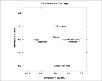
Correspondence analysis locates all the categories in a Euclidean space. The first two dimensions of this space are plotted to examine the associations among the categories. Since the smallest dimension of this table is three, there is no loss of information when only two dimensions are plotted. The plot should be thought of as two different overlaid plots, one for each categorical variable. Distances between points within a variable have meaning, but distances between points from different variables do not.
To interpret the plot, start by interpreting the row points separately from the column points. The European point is near and to the left of the centroid, so it makes a relatively small contribution to the chi-square statistic (because it is near the centroid), it contributes almost nothing to the inertia of dimension one (since its coordinate on dimension one has a small absolute value relative to the other column points), and it makes a relatively large contribution to the inertia of dimension two (since its coordinate on dimension two has a large absolute value relative to the other column points). Its squared cosines for dimension one and two, approximately 0 and 1, respectively, indicate that its position is almost completely determined by its location on dimension two. Its quality of display is 1.0, indicating perfect quality, since the table is two-dimensional after the centering. The American and Japanese points are far from the centroid, and they lie along dimension one. They make relatively large contributions to the chi-square statistic and the inertia of dimension one. The horizontal dimension seems to be largely determined by Japanese versus American car ownership.
In the row points, the Married point is near the centroid, and the Single with Kids point has a small coordinate on dimension one that is near zero. The horizontal dimension seems to be largely determined by the Single versus the Married with Kids points. The two interpretations of dimension one show the association with being Married with Kids and owning an American car, and being single and owning a Japanese car. The fact that the Married with Kids point is close to the American point and the fact that the Japanese point is near the Single point should be ignored. Distances between row and column points are not defined. The plot shows that more people who are married with kids than you would expect if the rows and columns were independent drive an American car, and more people who are single than you would expect if the rows and columns were independent drive a Japanese car.
Example 24.2. Multiple Correspondence Analysis of Cars and Their Owners
In this example, PROC CORRESP creates a Burt table from categorical data and performs a multiple correspondence analysis. The data are from a sample of individuals who were asked to provide information about themselves and their cars. The questions included origin of the car (American, Japanese, European), size of car (Small, Medium, Large), type of car (Family, Sporty, Work Vehicle), home ownership (Owns, Rents), marital/family status (single, married, single and living with children, and married living with children), and sex (Male, Female).
The data are read and formats assigned in a previous step, displayed in Example 24.1. The variables used in this example are Origin , Size , Type , Income , Home , Marital , and Sex . MCA specifies multiple correspondence analysis, OBSERVED displays the Burt table, and the OUTC= option creates an output coordinate data set. The TABLES statement with only a single variable list and no comma creates the Burt table. The %PLOTIT macro is used to plot the results with vertical and horizontal reference lines.
The data used to produce Output 24.2.1 and Output 24.2.2 can be found in Example 24.1.
| |
MCA of Car Owners and Car Attributes The CORRESP Procedure Burt Table American European Japanese Large Medium Small Family Sporty Work 1 Income American 125 0 0 36 60 29 81 24 20 58 European 0 44 0 4 20 20 17 23 4 18 Japanese 0 0 165 2 61 102 76 59 30 74 Large 36 4 2 42 0 0 30 1 11 20 Medium 60 20 61 0 141 0 89 39 13 57 Small 29 20 102 0 0 151 55 66 30 73 Family 81 17 76 30 89 55 174 0 0 69 Sporty 24 23 59 1 39 66 0 106 0 55 Work 20 4 30 11 13 30 0 0 54 26 1 Income 58 18 74 20 57 73 69 55 26 150 2 Incomes 67 26 91 22 84 78 105 51 28 0 Own 93 38 111 35 106 101 130 71 41 80 Rent 32 6 54 7 35 50 44 35 13 70 Married 37 13 51 9 42 50 50 35 16 10 Married with Kids 50 15 44 21 51 37 79 12 18 27 Single 32 15 62 11 40 58 35 57 17 99 Single with Kids 6 1 8 1 8 6 10 2 3 14 Female 58 21 70 17 70 62 83 44 22 47 Male 67 23 95 25 71 89 91 62 32 103 Burt Table Married Single 2 with with Incomes Own Rent Married Kids Single Kids Female Male American 67 93 32 37 50 32 6 58 67 European 26 38 6 13 15 15 1 21 23 Japanese 91 111 54 51 44 62 8 70 95 Large 22 35 7 9 21 11 1 17 25 Medium 84 106 35 42 51 40 8 70 71 Small 78 101 50 50 37 58 6 62 89 Family 105 130 44 50 79 35 10 83 91 Sporty 51 71 35 35 12 57 2 44 62 Work 28 41 13 16 18 17 3 22 32 1 Income 0 80 70 10 27 99 14 47 103 2 Incomes 184 162 22 91 82 10 1 102 82 Own 162 242 0 76 106 52 8 114 128 Rent 22 0 92 25 3 57 7 35 57 Married 91 76 25 101 0 0 0 53 48 Married with Kids 82 106 3 0 109 0 0 48 61 Single 10 52 57 0 0 109 0 35 74 Single with Kids 1 8 7 0 0 0 15 13 2 Female 102 114 35 53 48 35 13 149 0 Male 82 128 57 48 61 74 2 0 185 MCA of Car Owners and Car Attributes The CORRESP Procedure Inertia and Chi-Square Decomposition Singular Principal Chi- Cumulative Value Inertia Square Percent Percent 4 8 12 16 20 ----+----+----+----+----+--- 0.56934 0.32415 970.77 18.91 18.91 ************************ 0.48352 0.23380 700.17 13.64 32.55 ***************** 0.42716 0.18247 546.45 10.64 43.19 ************* 0.41215 0.16987 508.73 9.91 53.10 ************ 0.38773 0.15033 450.22 8.77 61.87 *********** 0.38520 0.14838 444.35 8.66 70.52 *********** 0.34066 0.11605 347.55 6.77 77.29 ******** 0.32983 0.10879 325.79 6.35 83.64 ******** 0.31517 0.09933 297.47 5.79 89.43 ******* 0.28069 0.07879 235.95 4.60 94.03 ****** 0.26115 0.06820 204.24 3.98 98.01 ***** 0.18477 0.03414 102.24 1.99 100.00 ** Total 1.71429 5133.92 100.00 Degrees of Freedom = 324 MCA of Car Owners and Car Attributes The CORRESP Procedure Column Coordinates Dim1 Dim2 American 0.4035 0.8129 European 0.0568 0.5552 Japanese 0.3208 0.4678 Large 0.6949 1.5666 Medium 0.2562 0.0965 Small 0.4326 0.5258 Family 0.4201 0.3602 Sporty 0.6604 0.6696 Work 0.0575 0.1539 1 Income 0.8251 0.5472 2 Incomes 0.6727 0.4461 Own 0.3887 0.0943 Rent 1.0225 0.2480 Married 0.4169 0.7954 Married with Kids 0.8200 0.3237 Single 1.1461 0.2930 Single with Kids 0.4373 0.8736 Female 0.3365 0.2057 Male 0.2710 0.1656 Summary Statistics for the Column Points Quality Mass Inertia American 0.4925 0.0535 0.0521 European 0.0473 0.0188 0.0724 Japanese 0.3141 0.0706 0.0422 Large 0.4224 0.0180 0.0729 Medium 0.0548 0.0603 0.0482 Small 0.3825 0.0646 0.0457 Family 0.3330 0.0744 0.0399 Sporty 0.4112 0.0453 0.0569 Work 0.0052 0.0231 0.0699 1 Income 0.7991 0.0642 0.0459 2 Incomes 0.7991 0.0787 0.0374 Own 0.4208 0.1035 0.0230 Rent 0.4208 0.0393 0.0604 Married 0.3496 0.0432 0.0581 Married with Kids 0.3765 0.0466 0.0561 Single 0.6780 0.0466 0.0561 Single with Kids 0.0449 0.0064 0.0796 Female 0.1253 0.0637 0.0462 Male 0.1253 0.0791 0.0372 MCA of Car Owners and Car Attributes The CORRESP Procedure Partial Contributions to Inertia for the Column Points Dim1 Dim2 American 0.0268 0.1511 European 0.0002 0.0248 Japanese 0.0224 0.0660 Large 0.0268 0.1886 Medium 0.0122 0.0024 Small 0.0373 0.0764 Family 0.0405 0.0413 Sporty 0.0610 0.0870 Work 0.0002 0.0023 1 Income 0.1348 0.0822 2 Incomes 0.1099 0.0670 Own 0.0482 0.0039 Rent 0.1269 0.0103 Married 0.0232 0.1169 Married with Kids 0.0967 0.0209 Single 0.1889 0.0171 Single with Kids 0.0038 0.0209 Female 0.0223 0.0115 Male 0.0179 0.0093 MCA of Car Owners and Car Attributes The CORRESP Procedure Indices of the Coordinates that Contribute Most to Inertia for the Column Points Dim1 Dim2 Best American 0 2 2 European 0 0 2 Japanese 0 2 2 Large 0 2 2 Medium 0 0 1 Small 0 2 2 Family 2 0 2 Sporty 2 2 2 Work 0 0 2 1 Income 1 1 1 2 Incomes 1 1 1 Own 1 0 1 Rent 1 0 1 Married 0 2 2 Married with Kids 1 0 1 Single 1 0 1 Single with Kids 0 0 2 Female 0 0 1 Male 0 0 1 Squared Cosines for the Column Points Dim1 Dim2 American 0.0974 0.3952 European 0.0005 0.0468 Japanese 0.1005 0.2136 Large 0.0695 0.3530 Medium 0.0480 0.0068 Small 0.1544 0.2281 Family 0.1919 0.1411 Sporty 0.2027 0.2085 Work 0.0006 0.0046 1 Income 0.5550 0.2441 2 Incomes 0.5550 0.2441 Own 0.3975 0.0234 Rent 0.3975 0.0234 Married 0.0753 0.2742 Married with Kids 0.3258 0.0508 Single 0.6364 0.0416 Single with Kids 0.0090 0.0359 Female 0.0912 0.0341 Male 0.0912 0.0341
| |
| |
| |
title 'MCA of Car Owners and Car Attributes'; *---Perform Multiple Correspondence Analysis---; proc corresp mca observed data=Cars outc=Coor; tables Origin Size Type Income Home Marital Sex; run; *---Plot the Multiple Correspondence Analysis Results---; %plotit(data=Coor, datatype=corresp, href=0, vref=0)
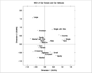
Multiple correspondence analysis locates all the categories in a Euclidean space. The first two dimensions of this space are plotted to examine the associations among the categories. The top-right quadrant of the plot shows that the categories single, single with kids, 1 income, and renting a home are associated. Proceeding clockwise, the categories sporty, small, and Japanese are associated. The bottom-left quadrant shows the association between being married, owning your own home, and having two incomes. Having children is associated with owning a large American family car. Such information could be used in market research to identify target audiences for advertisements.
This interpretation is based on points found in approximately the same direction from the origin and in approximately the same region of the space. Distances between points do not have a straightforward interpretation in multiple correspondence analysis. The geometry of multiple correspondence analysis is not a simple generalization of the geometry of simple correspondence analysis (Greenacre and Hastie 1987; Greenacre 1988).
If you want to perform a multiple correspondence analysis and get scores for the individuals, you can specify the BINARY option to analyze the binary table. In the interest of space, only the first ten rows of coordinates are printed.
title 'Car Owners and Car Attributes'; title2 'Binary Table'; *---Perform Multiple Correspondence Analysis---; proc corresp data=Cars binary; ods select RowCoors; tables Origin Size Type Income Home Marital Sex; run;
| |
Car Owners and Car Attributes Binary Table The Corresp Procedure Row Coordinates Dim1 Dim2 1 0.4093 1.0878 2 0.8198 0.2221 3 0.2193 0.5328 4 0.4382 1.1799 5 0.6750 0.3600 6 0.1778 0.1441 7 0.9375 0.6846 8 0.7405 0.1539 9 0.3027 0.2749 10 0.7263 0.0803
| |
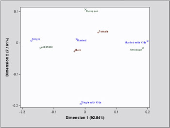
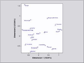
Example 24.3. Cars and Their Owners, ODS Graphics (Experimental)
These graphical displays are requested by specifying the experimental ODS GRAPHICS statement. For general information about ODS graphics, see Chapter 15, Statistical Graphics Using ODS. For specific information about the graphics available in the CORRESP procedure, see the ODS Graphics section on page 1109.
ods html; ods graphics on; *---Perform Simple Correspondence Analysis---; proc corresp short data=Cars; tables Sex Marital, Origin; supvar Sex; run; *---Perform Multiple Correspondence Analysis---; proc corresp mca short data=Cars; tables Origin Size Type Income Home Marital Sex; run; ods graphics off; ods html close;
| |
| |
| |
| |
Example 24.4. Simple Correspondence Analysis of U.S. Population
In this example, PROC CORRESP reads an existing contingency table with supplementary observations and performs a simple correspondence analysis. The data are populations of the fifty states, grouped into regions, for each of the census years from 1920 to 1970 (U.S. Bureau of the Census 1979). Alaska and Hawaii are treated as supplementary regions . They were not states during this entire period and they are not physically connected to the other 48 states. Consequently, it is reasonable to expect that population changes in these two states operate differently from population changes in the other states. The correspondence analysis is performed giving the supplementary points negative weight, then the coordinates for the supplementary points are computed in the solution defined by the other points.
The initial DATA step reads the table, provides labels for the years, flags the supplementary rows with negative weights, and specifies absolute weights of 1000 for all observations since the data were originally reported in units of 1000 people.
In the PROC CORRESP statement, PRINT=PERCENT and the display options display the table of cell percentages (OBSERVED), cell contributions to the total chi-square scaled to sum to 100 (CELLCHI2), row profile rows that sum to 100 (RP), and column profile columns that sum to 100 (CP). The SHORT option specifies that the correspondence analysis summary statistics, contributions to inertia, and squared cosines should not be displayed. The option OUTC=COOR creates the output coordinate data set. Since the data are already in table form, a VAR statement is used to read the table. Row labels are specified with the ID statement, and column labels come from the variable labels. The WEIGHT statement flags the supplementary observations and restores the table values to populations.
The %PLOTIT macro is used to plot the results. Normally, you only need to tell the %PLOTIT macro the name of the input data set, DATA= Coor , and the type of analysis performed on the data, DATATYPE=CORRESP. In this case, PLOTVARS= Dim1 Dim2 is also specified to indicate that Dim1 is the vertical axis variable, as opposed to the default PLOTVARS= Dim2 Dim1 .
For an essentially one-dimensional plot such as this, specifying PLOTVARS= Dim1 Dim2 improves the graphical display.
The following statements produce Output 24.4.1 and Output 24.4.2:
| |
United States Population The CORRESP Procedure Contingency Table Percents 1920 1930 1940 1950 1960 1970 Sum New England 0.830 0.916 0.946 1.045 1.179 1.328 6.245 NY, NJ, PA 2.497 2.946 3.089 3.382 3.833 4.173 19.921 Great Lake 2.409 2.838 2.987 3.410 4.064 4.516 20.224 Midwest 1.407 1.492 1.516 1.577 1.727 1.831 9.550 South Atlantic 1.569 1.772 1.999 2.376 2.914 3.441 14.071 KY, TN, AL, MS 0.998 1.109 1.209 1.284 1.352 1.436 7.388 AR, LA, OK, TX 1.149 1.366 1.466 1.631 1.902 2.167 9.681 Mountain 0.374 0.415 0.466 0.569 0.769 0.929 3.523 Pacific 0.625 0.919 1.092 1.625 2.282 2.855 9.398 Sum 11.859 13.773 14.771 16.900 20.020 22.677 100.000 Supplementary Rows Percents 1920 1930 1940 1950 1960 1970 Alaska 0.006170 0.006619 0.008189 0.014471 0.025353 0.033655 Hawaii 0.028719 0.041283 0.047453 0.056091 0.071011 0.086268 Contributions to the Total Chi-Square Statistic Percents 1920 1930 1940 1950 1960 1970 Sum New England 0.937 0.314 0.054 0.009 0.352 0.469 2.135 NY, NJ, PA 0.665 1.287 0.633 0.006 0.521 2.265 5.378 Great Lake 0.004 0.085 0.000 0.001 0.005 0.094 0.189 Midwest 5.749 2.039 0.684 0.072 1.546 4.472 14.563 South Atlantic 0.509 1.231 0.259 0.000 0.285 1.688 3.973 KY, TN, AL, MS 1.454 0.711 1.098 0.087 0.946 2.945 7.242 AR, LA, OK, TX 0.000 0.069 0.077 0.001 0.059 0.030 0.238 Mountain 0.391 0.868 0.497 0.098 0.498 1.834 4.187 Pacific 18.591 9.380 5.458 0.074 7.346 21.248 62.096 Sum 28.302 15.986 8.761 0.349 11.558 35.046 100.000 United States Population The CORRESP Procedure Row Profiles Percents 1920 1930 1940 1950 1960 1970 New England 13.2947 14.6688 15.1557 16.7310 18.8777 21.2722 NY, NJ, PA 12.5362 14.7888 15.5085 16.9766 19.2416 20.9484 Great Lake 11.9129 14.0325 14.7697 16.8626 20.0943 22.3281 Midwest 14.7348 15.6193 15.8777 16.5167 18.0825 19.1691 South Atlantic 11.1535 12.5917 14.2093 16.8872 20.7060 24.4523 KY, TN, AL, MS 13.5033 15.0126 16.3655 17.3813 18.2969 19.4403 AR, LA, OK, TX 11.8687 14.1111 15.1401 16.8471 19.6433 22.3897 Mountain 10.6242 11.7898 13.2166 16.1624 21.8312 26.3758 Pacific 6.6453 9.7823 11.6182 17.2918 24.2784 30.3841 Supplementary Row Profiles Percents 1920 1930 1940 1950 1960 1970 Alaska 6.5321 7.0071 8.6698 15.3207 26.8409 35.6295 Hawaii 8.6809 12.4788 14.3438 16.9549 21.4649 26.0766 Column Profiles Percents 1920 1930 1940 1950 1960 1970 New England 7.0012 6.6511 6.4078 6.1826 5.8886 5.8582 NY, NJ, PA 21.0586 21.3894 20.9155 20.0109 19.1457 18.4023 Great Lake 20.3160 20.6042 20.2221 20.1788 20.2983 19.9126 Midwest 11.8664 10.8303 10.2660 9.3337 8.6259 8.0730 South Atlantic 13.2343 12.8641 13.5363 14.0606 14.5532 15.1729 KY, TN, AL, MS 8.4126 8.0529 8.1857 7.5985 6.7521 6.3336 AR, LA, OK, TX 9.6888 9.9181 9.9227 9.6503 9.4983 9.5581 Mountain 3.1558 3.0152 3.1519 3.3688 3.8411 4.0971 Pacific 5.2663 6.6748 7.3921 9.6158 11.3968 12.5921 United States Population The CORRESP Procedure Inertia and Chi-Square Decomposition Singular Principal Chi- Cumulative Value Inertia Square Percent Percent 20 40 60 80 100 ----+----+----+----+----+--- 0.10664 0.01137 1.014E7 98.16 98.16 ************************* 0.01238 0.00015 136586 1.32 99.48 0.00658 0.00004 38540 0.37 99.85 0.00333 0.00001 9896.6 0.10 99.95 0.00244 0.00001 5309.9 0.05 100.00 Total 0.01159 1.033E7 100.00 Degrees of Freedom = 40 Row Coordinates Dim1 Dim2 New England 0.0611 0.0132 NY, NJ, PA 0.0546 0.0117 Great Lake 0.0074 0.0028 Midwest 0.1315 0.0186 South Atlantic 0.0553 0.0105 KY, TN, AL, MS 0.1044 0.0144 AR, LA, OK, TX 0.0131 0.0067 Mountain 0.1121 0.0338 Pacific 0.2766 0.0070 Supplementary Row Coordinates Dim1 Dim2 Alaska 0.4152 0.0912 Hawaii 0.1198 0.0321 Column Coordinates Dim1 Dim2 1920 0.1642 0.0263 1930 0.1149 0.0089 1940 0.0816 0.0108 1950 0.0046 0.0125 1960 0.0815 0.0007 1970 0.1335 0.0086
| |
| |
| |
title 'United States Population'; data USPop; * Regions: * New England - ME, NH, VT, MA, RI, CT. * Great Lake - OH, IN, IL, MI, WI. * South Atlantic - DE, MD, DC, VA, WV, NC, SC, GA, FL. * Mountain - MT, ID, WY, CO, NM, AZ, UT, NV. * Pacific - WA, OR, CA. * * Note: Multiply data values by 1000 to get populations.; input Region . y1920 y1930 y1940 y1950 y1960 y1970; label y1920 = '1920' y1930 = '1930' y1940 = '1940' y1950 = '1950' y1960 = '1960' y1970 = '1970'; if region = 'Hawaii' or region = 'Alaska' then w = -1000; /* Flag Supplementary Observations */ else w = 1000; datalines; New England 7401 8166 8437 9314 10509 11842 NY, NJ, PA 22261 26261 27539 30146 34168 37199 Great Lake 21476 25297 26626 30399 36225 40252 Midwest 12544 13297 13517 14061 15394 16319 South Atlantic 13990 15794 17823 21182 25972 30671 KY, TN, AL, MS 8893 9887 10778 11447 12050 12803 AR, LA, OK, TX 10242 12177 13065 14538 16951 19321 Mountain 3336 3702 4150 5075 6855 8282 Pacific 5567 8195 9733 14486 20339 25454 Alaska 55 59 73 129 226 300 Hawaii 256 368 423 500 633 769 ; *---Perform Simple Correspondence Analysis---; proc corresp print=percent observed cellchi2 rp cp short outc=Coor; var y1920 -- y1970; id Region; weight w; run; *---Plot the Simple Correspondence Analysis Results---; %plotit(data=Coor, datatype=corresp, plotvars=Dim1 Dim2)
The contingency table shows that the population of all regions increased over this time period. The row profiles show that population is increasing at a different rate for the different regions. There is a small increase in population in the Midwest, for example, but the population has more than quadrupled in the Pacific region over the same period. The column profiles show that in 1920, the US population was concentrated in the NY, NJ, PA, Great Lakes, Midwest, and South Atlantic regions. With time, the population is shifting more to the South Atlantic, Mountain, and Pacificregions. This is also clear from the correspondence analysis. The inertia and chi-square decomposition table shows that there are five nontrivial dimensions in the table, but the association between the rows and columns is almost entirely one-dimensional.
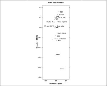
The plot shows that the first dimension correctly orders the years. There is nothing in the correspondence analysis that forces this to happen; PROC CORRESP knows nothing about the inherent ordering of the column categories. The ordering of the regions and the ordering of the years reflect the shift over time of the U.S. population from the Northeast quadrant of the country to the South and to the West. The results show that the West and Southeast are growing faster than the rest of the contiguous 48 states.
The plot also shows that the growth pattern for Hawaii is similar to the growth pattern for the mountain states and that Alaska s growth is even more extreme than the Pacific states growth. The row profiles confirm this interpretation.
The Pacific region is farther from the origin than all other active points. The Midwest is the extreme region in the other direction. The table of contributions to the total chi-square shows that 62% of the total chi-square statistic is contributed by the Pacific region, which is followed by the Midwest at over 14%. Similarly the two extreme years, 1920 and 1970, together contribute over 63% to the total chi-square, whereas the years nearer the origin of the plot contribute less.