Creating Amortization Schedules

In its simplest form, an amortization schedule tracks the payments (including interest and principal components) and the loan balance for a particular loan. This section presents several examples of amortization schedules.

A Simple Amortization Schedule

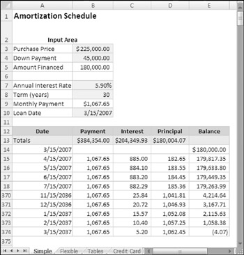
This example uses a simple loan to demonstrate the basic concepts involved in creating a dynamic schedule. Refer to the worksheet in Figure 13-1. Notice that rows 19 through 369 are hidden, so only the first five payments and last five payments are visible.

Figure 13-1: A simple amortization schedule.

On the CD 

All the examples in this section are available on the companion CD-ROM in the workbook  amortization.xlsx.

USER INPUT SECTION

The area above the schedule contains cells for user input and for intermediate calculations. The user input cells are shaded, so it's easy to determine what can be changed and what has a formula.

The user can enter the purchase price and the down payment. The amount financed is calculated for use in the amortization calculation. The formula in cell B5 is

 =Purchase_Price-Down_Payment 

Tip 

Descriptively named ranges are used to make the formulas more readable.

The other calculation necessary to complete the schedule is the monthly payment. The formula in B9 is

 =-ROUND(PMT(Rate/12,Term*12,Amount_Financed),2) 

Cross Ref 

More information on named cells and ranges is in Chapter 3.

The PMT function is used to determine the monthly payment amount. The rate (B7) is divided by 12, and the term (B8) is multiplied by 12, so that the arguments are on a monthly basis. This ensures that the result of PMT is also on a monthly basis.

The ROUND function rounds the result of PMT to two decimal places. t is an attractive proposition not to round this number so that the result is accurate to the penny. However, because you will not be paying the bank fractions of pennies, you shouldn't have them in your schedule.

SUMMARY INFORMATION

The first line of the schedule, after the header information, contains summary formulas. In this example, only the totals are shown. However, you could include totals by year, quarter, or any other interval you like. The formula in B13, and copied across, is

 =SUM(B14:B381) 

Tip 

Placing the summary information above the schedule itself eliminates the need to scroll to the end of the worksheet.

THE SCHEDULE

The schedule starts in row 14 with the amount financed as the beginning balance. The first payment is deemed to be made exactly one month after the loan is initiated. The first payment row (row 15) and all subsequent rows contain the same formulas, which are described below. The formula in E14 is

 =Amount_Financed 

To increment the date for the payment rows, the DATE function is used. The formula in A15 is

 =DATE(YEAR(A14),MONTH(A14)+1,DAY(A14)) 

The DATE function constructs a date from the year, month, and day arguments. The arguments are derived from the cell above, and the month is increment by one.

The payment column simply references the PMT function from the user input section. Because that formula was rounded, no further rounding is necessary.

The interest column computes a monthly interest based on the previous balance. The formula in C15 is

 =ROUND(E14*Rate/12,2) 

The previous balance, in cell E14, is multiplied by the annual interest rate which is divided by 12. The annual interest rate is in cell B7, named Rate. Each month's balance must be rounded to the penny, so every interest calculation is rounded as you go.

Whatever portion of the payment doesn't go toward interest goes toward reducing the principal balance. The formula in D15 is

 =B15-C15 

Finally, the balance is updated to reflect the principal portion of the payment. The formula in E15 is

 =E14-D15 

Loan amortization schedules are self-checking. If everything is set up correctly, the final balance at the end of the term is 0 (or very close to 0, given rounding errors).

Tip 

Another check is to add the Principal components. The sum of these values should equal the original loan amount.

LIMITATIONS

This type of schedule is excellent for loans that will likely never change. It can be set up one time and referred to throughout the life of the loan. Further, it can be copied to create new loan with just a few adjustments. However, it leaves a little to be desired.

You may have noticed that the balance at the end of the loan, as well as the total principal paid in the summary section, is off by $4.07. This is because of the rounding of each month's payment and interest calculation. Although rounding those results is necessary, a more flexible schedule would allow you to adjust the final payment so the balance is zero when the final payment is made.

This schedule lacks flexibility in other ways as well:

• The payment is computed and applied every month but cannot account for over or under-payments.

• Many loans have variable interest rates, and this schedule provides no way to adjust the interest rate per period.

• Although the user is allowed to specify a term, the rows in the schedule are fixed. Specifying a shorter or longer term would require that formulas be deleted or added to compensate.

In the next section, I address some of the flexibility issues and create a more dynamic amortization schedule.

A Dynamic Amortization Schedule

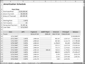
The example in this section builds on the previous example. Figure 13-2 shows a loan amortization schedule that allows the user to define input parameters beyond the amount, rate, and term. Notice that rows 22 through 124 are hidden.

Figure 13-2: A dynamic amortization schedule.

The first difference you'll notice is that this schedule has more shaded cells, meaning there are more cells that the user can change. Also, a column has been added for the annual percentage rate, which now can be different for every period.

USER INPUT SECTION

Not much has changed in this section. The interest rate is labeled Starting Rate, and the payment is labeled Computed Payment, indicating that they are subject to change.

SUMMARY INFORMATION

The user can now change the term; the interest rates; and the payments, which can and usually will change the maturity date. For the summary information, you want to sum only the relevant rows. The formula in C13 is

 =SUMIF($F15:$F374,">=0",C15:C374) 

After the Balance in column F is zero, the amortization is complete. This SUMIF function sums only those payments up until that point. This formula is copied across to the interest and principal columns, and the absolute column reference ensures the new formulas still point to column F.

THE SCHEDULE

With so many user changeable fields in the schedule, many of the formulas had to change to account for different conditions. An amortization schedule has two kinds of user input data:

• Data that changes for one payment only

• Data that changes for all subsequent payments

When the interest rate changes for one payment, it changes for all subsequent payment-at least, until it changes again. It doesn't go back to the old rate. For that reason, the APR column relies on the data directly above it. The formula in B15 pulls the starting interest rate from the user input section. This formula, in B16 and copied down, simply repeats the previous month's rate:

 =B15 

This allows the user to enter a new rate when it changes and have that rate continue down until it's manually changed again. In this example, the bank informed you that the rate was reduced to 4.8% for the fifth payment (row 19). That rate was entered in B19, and all rates after that reflect the change.

The payment date is an example of data that changes for one payment. If a payment is made late, it doesn't mean that all subsequent payments will be late. In this example, the third payment (row 17) was made ten days late. This had no effect on the next month's payment, which was made on time. For this type of data, the increments need to be made against a base that doesn't change. The formula in A15 is

 =DATE(YEAR(Loan_Date),MONTH(Loan_Date)+ROW()-14,DAY(Loan_Date)) 

This formula is copied down to all the rows. Unlike the previous example, it doesn't rely on the date above it. Rather, it uses the Loan_Date range as its base. Because the payments start in row 15, the current row less 14 is used to increment the month.

The point of these formulas is to allow the user to overwrite the formula with a literal date value and not affect the rest of the dates. In Cell A17, the user replaced the formula by entering a new date, which changed the calculation for that payment but did not affect future payments.

Because you provide a separate column for an additional payment, the payment should never change-except that it needs to account for any previous rounding errors in the last payment. The formula in C15 is

 =IF(G127+E128-Monthly_Payment-D128<5,G127+E128-D128,Monthly_Payment) 

Normally, if the remaining balance is less than the normal payment, just the balance (plus interest) is paid. However, in this example, I don't want a last payment of less than $5. If a normal payment would leave such a balance, it is just added to the last payment. There's nothing wrong with a really small final payments. If you don't mind them, you can simplify the formula to

 =IF(G127+E128<Monthly_Payment+D128,G127+E128-D128,Monthly_Payment) 

The interest calculation now has to account for the fact that the user may make a payment early or late. Instead of dividing the rate by 12, as in the last example, the rate is multiplied by a ratio of the number of days outstanding to 365. The formula in E15 is

 =ROUND(G14*B15*(A15-A14)/365,2) 

The principal column calculation is similar to the previous example except that any additional payment must be added in. The formula in F15 is

 =C15+D15-E15 

The balance is computed by subtracting the principal portion of the current payment from the previous balance, exactly as it was in the previous example.

FINISHING TOUCHES

As you can see in Figure 13-2 (which hides rows in the middle so you can see the last payment), the final payment is represented in row 127, and there are no calculations below that. I didn't just guess right, however. All the cells in the schedule, starting in row 15, have conditional formatting applied to them. If column G of the row above is zero or less, both the background color and the font color are white, rendering them invisible.

To apply conditional formatting, select the range A15:G374 and choose the Home Styles Conditional Formatting command. Add a formula rule with this formula:

 =$G14<=0 

The absolute column means that every column in the selection will refer to column G; the relative row means the row applies to the row above, regardless of which row you're in.

Cross Ref 

For more information on conditional formatting, refer to Chapter 19.

The formulas are present in row beyond row 127 (they exist for up to 360 months) but are hidden using conditional formatting to make the table size dynamic as well.

Using Payment and Interest Tables

The preceding example allows the user to input data directly in the calculation and reporting section of the schedule. This affords maximum flexibility and adds a level of intuitiveness to customizing the schedule. Depending on the intended user, however, it could be dangerous and lead to errors. In particular, overwriting formulas, like changing the interest rate in the last example, does not lend itself to undoing or correcting errors. Unless the user is intimately familiar with the workings of the spreadsheet, those hard-coded values can stick around when the user thinks they're formulas.

Another method-and some would argue a better method-is to keep the user input section separate from the calculation and report section. If all user inputs are relegated to one area, it's easier to determine what has been inputted and whether any inputs are missing.

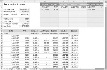
This example uses the same basic data as the previous two examples. It adds an additional payment table, an interest rate table, and a late payment table in the user input\section, and the formulas are adjusted. Figure 13-3 shows the user input section of this flexible schedule.

Figure 13-3: Keeping the user input isolated in its own area.

Nothing in the schedule can be updated by the user. Changes to the amortization table must be made in the inputs in column B or in one of the three tables to the right of that. The new formulas in the schedule are discussed in the following sections. Formulas not listed have not changed from the previous example.

DATE

 =DATE(YEAR(Loan_Date),MONTH(Loan_Date)+ROW()-14, DAY(Loan_Date))+IFERROR(VLOOKUP(DATE(YEAR(Loan_Date), MONTH(Loan_Date)+ROW()-14,DAY(Loan_Date)),tblLate,2,FALSE),0) 

This formula looks a little daunting, but it's not too bad. It starts with the same DATE function used in the preceding example and adds the number of late days from tblLate. The VLOOKUP function looks for an exact match in the first column of tblDate; the number in the second column, either plus or minus, is added to the originally computed date. The IFERROR function is used to return a zero if no match is found, meaning the originally computed date is used.

APR

 =IFERROR(VLOOKUP(A15,tblRate,2),Rate) 

The table tblRate contains a list of interest rate changes. The VLOOKUP function is used with an omitted fourth argument so that the rate change persists until it is changed again. This means that the dates in tblRate must be sorted.

The IFERROR statement returns the starting rate if no value is found in tblRate.

ADDITIONAL PAYMENT

 =SUMIFS(tblAdd[Add_Amt],tblAdd[Add_Start], "<="&A15,tblAdd[Add_End],">="&A15) 

The table tblAdd is a listing of additional payments, the date they become effective, and the date they expire. To add a one-time additional payment, the user can make the start and end dates the same. To schedule a series of additional payments, however, this method allows the user to add them quickly. The SUMIFS formula adds the additional amount for every row in the table where the current payment date is in between the start and end dates. That means that more than one additional payment can be made for one date.

Cross Ref 

You can find more information on referring to tables in formulas in Chapter 9. Summing and counting functions, like SUMIFS, are discussed in Chapter 7. And examples of lookup functions, such as VLOOKUP, as well as the IFERROR function are given in Chapter 8.

Credit Card Calculations

The final type of loan amortization schedule is for credit card loans. Credit cards are different beasts because the minimum payment varies, based on the outstanding balance. You could use the preceding Payment Table method, but it offers only nine rows of varying payments–probably not enough for most applications. You could also use the method where the payments are entered directly in the schedule. When the payments are different every time, however, the schedule loses its value as a predictor or planner. You need a schedule that can predict the future payments of a credit card loan.

Credit card calculations represent several nonstandard problems. Excel's financial functions (PV, FV, RATE, and NPER) require that the regular payments are at a single level. In addition, the PMT function returns a single level of payments. With IRR and NPV analysis, the user inserts the varying payments into a cash flow.

Credit card companies calculate payments based on the following relatively standard set of criteria:

• A minimum payment is required. For example, a credit card account might require a minimum payment of $25.

• The payment must be at least equal to a base percentage of the outstanding debt. Usually, the payment is a percentage of the outstanding balance but not less than a specified amount.

• The payment is rounded, usually to the nearest $0.05.

• Interest is invariably quoted at a given rate per month.

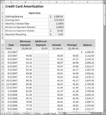
Figure 13-4 shows a worksheet set up to calculate credit card payments.

Figure 13-4: Calculating a credit card payment schedule.

The formula for the minimum payment is rather complicated-just like the terms of a credit card. This example uses a minimum payment amount of $25 or 3% of the balance, which results in a very long payback. If this borrower ever hopes to get rid of that balance in a reasonable amount of time, he'll need to use that additional payment column.

The minimum payment formula, such as the one in B13, is

 =MIN(F12+D13,MROUND(MAX(MinDol,ROUND(MinPct*F12,2)),PayRnd)) 

From the inside out: The larger of the minimum dollar amount and the minimum percent is calculated. The result of that is rounded to the nearest five cents. This rounded amount is then compared with the outstanding balance, and the lesser of the two is used.

Of course, things get much more complicated when additional charges are made. In such a case, the formulas would need to account for "grace periods" for purchases (but not cash withdrawals). A further complication is that interest is calculated on the daily outstanding balance at the daily effective equivalent of the quoted rate.