Limitations of Excel s Financial Functions | Excel 2007 Formulas (Mr. Spreadsheets Bookshelf)

Limitations of Excel's Financial Functions

Excel's primary financial functions (PV, FV, PMT, RATE, NPER, CUMIPMT, and CUMPRINC) are very useful, but they have two common limitations:

They can handle only one level of interest rate.
They can handle only one level of payment.

For example, the NPER function cannot handle the variations in payments that arise with credit card calculations. In such calculations, the monthly payment is based upon a reducing outstanding balance and may also be subject to a minimum amount rule.

The common solution to the problem of varying payments is to create a cash flow schedule and use other financial functions that can handle multiple payments and rates. Examples of the process appear in the next two chapters. Briefly, the functions involved are

FVSCHEDULE, which calculates a future value when the interest rate is variable
IRR, which calculates a rate of return from a varying level of cash flow received at regular intervals
NPV, which calculates the sum of the present values of a varying level of cash flow received at regular intervals
MIRR, which is a modified IRR that considers cash flows that are reinvested
XIRR, which calculates a single rate from irregular cash flows
XNPV, which calculates the net present value of irregular cash flows

In a situation that involves only slight variations, you can combine and nest Excel's financial functions.

On the CD

The examples in this section can be found in the file named extending basic functions.xlsx on the companion CD-ROM.

Deferred Start to a Series of Regular Payments

In some cases, a series of cash flows may have a deferred start. You can calculate the PV of a regular series of cash flows with a deferred start by nesting PV functions.

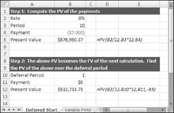
In this example, you get a loan to start a business. You can afford to pay $7,000 per month, and you negotiate a deal with the bank to defer the first payment for 12 months. If the bank quotes an 8% rate on a ten-year loan, this formula will tell you how much you can borrow (see Figure 11-16):

 =PV(0.08/12,12,0,-PV(0.08/12,10*12,-7000))

image from book
Figure 11-16: Calculating the present value of regular payments with a deferred start is a two-step process.

First, calculate the present value, which is $576,950. This value is used as the future value argument of the outer function. The outer function further discounts this amount over the year deferral period, and results in $532,733. In other words, if you borrow $532,733 now, the amount will increase to $576,950 in one year with no payments, and it will reduce to zero in ten years with a $7,000 monthly payment.

Valuing a Series of Variable Payments

This example calculates the present value when the payments change over time. Assume that you want to buy your way out of a property lease, and you need to know how much it's worth. There's nine years left on the lease, and the payment schedule is

Years 1–3: $5,000/month
Years 4– 6: $6,500/month
Years 7– 9: $8,500/month

The following formula will calculate the value of the lease assuming a 10% discount rate:

 =PV(.1/12,36,-5000)+ PV(.1/12,3*12,0,-PV(.1/12,36,-6500))+ PV(.1/12,6*12,0,-PV(.1/12,36,-8500))

The result of $449,305 is calculated in three steps:

Compute the present value of three years of rent payments.
The second three years is the same as the preceding deferred start example. The present value of its payments are computed, and that becomes the future value argument to a different PV function. That future value is discounted over a three year deferred period (while the $5,000 rent payments are being made).
The last three years of payments are similarly discounted but this time over a six-year deferral period.