Nonlinear Profit Analysis

[Page 452 ( continued )]

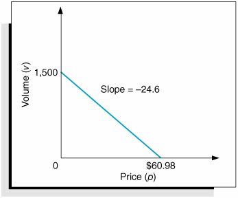
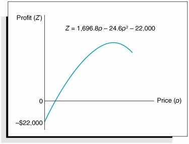
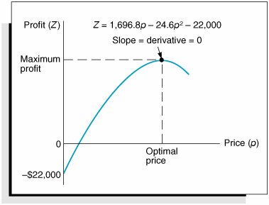
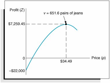
We begin our presentation of nonlinear programming models by determining the optimal value for a single nonlinear function. To demonstrate the solution procedure, we will use a profit function based on break-even analysis. In Chapter 1 we used break-even analysis to begin our study of model building, so it seems appropriate that we return to this basic model to complete our study of model building.

Recall that in break-even analysis the profit function, Z , is formulated as

Z = vp c _f vc _v

where

v = sales volume (i.e., demand)

p = price

c _f = fixed cost

c _v = variable cost

One important but somewhat unrealistic assumption of this break-even model is that volume, or demand, is independent of price (i.e., volume remains constant, regardless of the price of the product). It would be more realistic for the demand to vary as price increased or decreased. For our Western Clothing Company example from Chapter 1, let us suppose that the dependency of demand on price is defined by the following linear function:

---

[Page 453]

v = 1,500 24.6 p

This linear relationship is illustrated in Figure 10.1. The figure illustrates the fact that as price increases , demand decreases, up to a particular price level ($60.98) that will result in no sales volume.

Figure 10.1. Linear relationship of volume to price

Now we will insert our new relationship for volume ( v ) into our original profit equation:

Substituting values for fixed cost ( c _f = $10,000) and variable cost ( c _v = $8) into this new profit function results in the following equation:

Because of the squared term , this equation for profit is now a nonlinear, or quadratic, function that relates profit to price, as shown in Figure 10.2.

Figure 10.2. The nonlinear profit function

---

[Page 454]

In Figure 10.2, the greatest profit will occur at the point where the profit curve is at its highest. At that point the slope of the curve will equal zero, as shown in Figure 10.3.

Figure 10.3. Maximum profit for the profit function

In calculus the slope of a curve at any point is equal to the derivative of the mathematical function that defines the curve. The derivative of our profit function is determined as follows :

The slope of a curve at any point is equal to the derivative of the curve's function .

Given this derivative, the slope of the profit curve at its highest point is defined by the following relationship:

0 = 1,696.8 49.2 p

The slope of a curve at its highest point equals zero .

Now we can solve this relationship for the optimal price, p , which will maximize total profit:

The optimal volume of denim jeans to produce is computed by substituting this price into our previously developed linear relationship for volume:

The maximum total profit is computed as follows:

The maximum profit, optimal price, and optimal volume are shown graphically in Figure 10.4.

---

[Page 455]

Figure 10.4. Maximum profit, optimal price, and optimal volume

An important concept we have yet to mention is that by extending the break-even model this way, we have converted it into an optimization model. In other words, we are now able to maximize an objective function (profit) by determining the optimal value of a variable (price). This is exactly what we did in linear programming when we determined the values of decision variables that optimized an objective function. The use of calculus to find optimal values for variables is often referred to as classical optimization .

Classical optimization is the use of calculus to determine the optimal value of a variable .