PROBABILITY CONCEPTS

• Probability quantifies the chances an event will occur.

• Bound probability of an event A.

  ‰ P(A) ‰ 1

• Probability of an event A that is certain to occur.

  P(A) = 1

  [100%]

• Probability of an event A that cannot occur.

  P(A) = 0

  [0%]

1. Estimates of probability

   1. Classical or a- priori approach ” This approach is based on "equally likely" events.

      • Assumes all simple events or individual outcomes are "equally likely."

      • Sample space S: A random experiment with a total of n possible outcomes.

      • Defined event A: Has r of these possible outcomes [r ‰ n].

      • Probability of event A: P(A) =

   Example 1

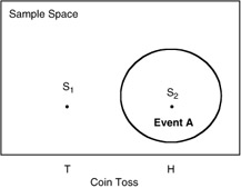
   Random experiment: Single toss of one coin.

   Find: Probability of a head.

   Sample space: S = {S ₁ , S ₂ } = {T, H}.

   TWO mutually exclusive events: n = 2.

   Event A: Tossing ONE head S ₂ ; r = 1.

   Assume each outcome is "equally likely."

   Probability of Event A = S ₂ : P(A) = P(S ₂ ) = r/n = 1/2

   
    

   Example 2

   Random experiment: Twice-tossed coin.

   Find: Probability of two heads.

   Sample space: S = {S ₁ , S ₂ , S ₃ , S ₄ } = {TT, TH, HT, HH}

   FOUR mutually exclusive events: n = 4.

   S ₁ = TT, S ₂ = TH, S ₃ = HT, S ₄ = HH

   Event A: Tossing TWO heads, which is simple event S ₄ ; r = 1.

   Assume the four possible outcomes are "equally likely."

   Probability of Event A = S ₄ : P(A) = P(S ₄ ) = r/n = 1/4

    

   Example 3

   Random Experiment: Single roll of fair die.

   Find: Probability of rolling a 3.

   Sample space: S = {S ₁ , S ₂ , S ₃ , S ₄ , S ₅ , S ₆ } = {1, 2, 3, 4, 5, 6}

   SIX mutually exclusive simple events: n = 6.

   Event A: Rolling the ONE number 3 on the die (i.e., S ₃ ); r = 1.

   Assume each of the six possible outcomes is "equally likely.

   " Probability of Event A = S ₃ : P(A) = P(S ₃ ) = r/n = 1/6

   2. Frequency or a-posteriori approach ” This approach is based on a "very large" number of independent samples.

      • Assumes after n repetitions of a given random experiments, a simple event S _i is observed to occur in r _i of these.

      • Assumes n is "very large."

      • Vague about how "large" n must be.

      • Empirical probability: P(A) = P(S _i ) ‰ˆ

    

   Example 4

   Random Experiment: Tossing a single coin.

   Sample space: S = {S ₁ , S ₂ } = {T, H}

   TWO mutually exclusive events: n = 2

   Event A: The simple event S ₂ (head) will occur.

   Observations: After n = 1000 tosses we find we have accumulated 483 heads and 517 tails .

   Empirical probability of the event "a head:"

   P(A) = P(S ₂ ) ‰ˆ = 0.483

   Special note:  

   This is not the same as the 0.5 of the classical approach (Example 1).

    

   3. Axiomatic approach ” This approach is based on set theory.

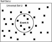
      Rule 1: Probability of an event A is bounded.

      ‰ P(A) ‰ 1

      • Certainty or the sure occurrence of event A

      • Using Sets: Event A = Sample Space S

        P(A) = P(S) = 1

      • Impossibility or absence of the event A

      • Using Sets: Event A = Null Space

        P(A) = P( ) = 0

        

      Rule 2: Total or cumulative probability

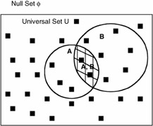
      • P(A ‹ƒ B) = P(A) + P(B) - P(A ‹‚ B)

      • "OR"

      • P(A + B) = P(A) + P(B) - P(A · B)

      • P(A + B) = probability of either events A or B or both

      • P(A) = probability of event A alone

      • P(B) = probability of event B alone

      • P(A ‹‚ B) = probability of both events A and B

      • "AND" implies intersection of sets: (A ‹‚ B) = (A · B), in other words, it removes one count of common simple events.

        

      • Useful alternate form: P(A + B) = 1 - P(A* B*)

      • Similarly, with THREE EVENTS (parallel components of "OR" events)

        P(A ‹ƒ B ‹ƒ C) = P(A) + P(B) + P(C) - P(A ‹‚ B) - P(A ‹‚ C) - P(B ‹‚ C) + P(A ‹‚ B ‹‚ C)

      Rule 2A: Total probability of MUTUALLY EXCLUSIVE EVENTS (not to be confused with independent events). In this case, the occurrence of one event precludes the occurrence of another.

      Sets: Events A and B are mutually exclusive if they have no common simple event.

      "AND" intersection set is zero: A ‹‚ B = 0

      Hence, P(A + B) = Probability of either events A or B or both becomes the sum of the individual probabilities:

      P(A + B)	=	P(A ‹ƒ B)
      	=	P(A) + P(B) - P(A ‹‚ B)
      	=	P(A) + P(B)

      

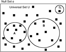
      Note  

      All individual simple events, S _i , are mutually exclusive.

   Example 5

   Random Experiment: A single toss of a fair die.

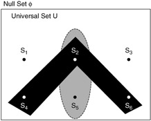
   Sample space: Six "equally likely" simple events

   S ₁ = 1, S ₂ = 2, S ₃ = 3, S ₄ = 4, S _s = 5, S ₆ = 6

   Event A: Defined as either a 2 or 5 will occur.

   A = {S ₂ , S ₅ }

   Event B: Defined as any even number will occur.

   B = {S ₂ , S ₄ , S ₆ }

   Probability of individual event:

   P(S _i ) = 1/6; I = 1, 2, ... 6

   Probability of Event A:

   P(A) = P(S ₂ + S ₅ ) = P(S ₂ ) + P(S ₅ )

   

   Probability of Event B:

   P(B) = P(S ₂ + S ₄ + S ₆ ) = P(S ₂ ) + P(S ₄ ) + P(S ₆ )

   
   
    

   Example 5A

   Random Experiment: A single toss of a fair die.

   Find: Total probability that the events A or B or both occur.

   "OR" total probability

   P(A + B) = P(A) + P(B) - P(A, B)

   where P(A) = 1/3; P(B) = 1/2

   P(A, B) = probability of both events A and B = P(S ₂ ) = 1/6

   P(A + B) = 1/3 + 1/2 - 1/6 = 4/6 = 2/3

   

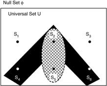
   Note  

   Total probability must be greater or equal than that of A or B alone.

   Rule 3: Joint and Conditional Probability

   • Joint probability: Probability that an outcome will satisfy both events A and B simultaneously .

     P(A B) = P(A ‹‚ B)	=	P(A)P(B A)
     	=	P(B)P(A B)

   • Conditional Probability: Probability of A given B

   • P(A B) = Probability of A given that B has occurred

     

   Rule 3A: Joint probability of mutually exclusive events. Mutually exclusive is not the same as independent.

   • Joint probability of two mutually exclusive events A and B:

     P(A B) ‰ P(A ‹‚ B) = 0

   • Conditional probability of two mutually exclusive events is undefined since by definition the occurrence of event B excludes the occurrence of event A (see Bayes' Rule).

   • For THREE EVENTS (multiplication)

   P(A · B · C) = P(A ‹‚ B ‹‚ C)	=	P(A)P(B A)P(C A ‹‚ B)
   	=	P(A)P(B)P(C) if independent

   Rule 4: Independent events. Events such that the occurrence of one has no effect on the occurrence of another.

   • Conditional probability of independent events:

     P(A B) = P(A)

   • Joint probability of independent events:

     P(A · B) = P(A ‹‚ B) = P(A)P(B A) = P(A)P(B)

     This actually turns out to be the definition of "independence" of events.

     

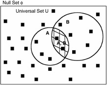
     The reader should note that since both P(A) and P(B) are less than unity, their product will be smaller than either.

     (e.g., 1/4 — 1/3 = 1/12)

     Therefore, the total probability of independent events may be shown as:

     P(A ‹ƒ B)	‰	P(A) + P(B) - P(A ‹‚ B)
     	=	P(A) + P(B) - P(A)P(B A)
     	=	P(A) + P(B) - P(A)P(B)

    

   Example 5B

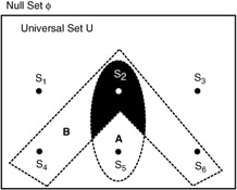
   Random Experiment: A single toss of a fair die

   Find: Joint probability that events A and B occur

   P(A · B) = P(A)P(B A)

   Independent Events: Events A and B are independent since each consists of a set of the independent sample space S.

   Mutually Exclusive Events: Events A and B are not mutually exclusive since they have one common simple event S ₂ .

   P(A · B) = P(A)P(B A)	=	P(A)P(B)
   	=	1/3 — 1/2 = 1/6

   
    

   Example 6

   Random Experiment: A single toss of a fair die and a coin.

   Sample Space: Twelve "equally likely" simple events.

   

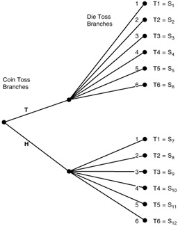
   Sample Space S: Twelve "equally likely" simple events

   P(S _i ) = 1/12; i = 1, 2, ..., 12

   Event A: Coin is a head and die has an even number

   A = {S ₈ , S ₁₀ , S ₁₂ }

   P(A) = P(S ₈ ) + P(S ₁₀ ) + P(S ₁₂ ) = 1/12 + 1/12 + 1/12 = 1/4

   Event B: Any coin toss and die less than 5 (i.e., 1, 2, 3, 4)

   B = {S ₁ , S ₂ , S ₃ , S ₄ , S ₇ , S ₈ , S ₉ , S ₁₀ }

   P(B) = 8P(S _i ) = 8/12 = 2/3

    

   Example 6A

   Random Experiment: A single toss of a fair die and a coin.

   Find: Joint probability of independent events A and B.

   Joint probability that A and B occur

   P(A - B) = P(A)P(B A)

   Independent Events: Events A and B are assumed independent; the probability of event B given that A has occurred is simply

   P(B A) = P(B)

   Joint probability of the given independent events is

   P(A · B) = P(A)P(B) = 1/4 · 2/3 = 2/12 = 1/6

   Note  

   Since both events must occur, probability of "success" will be smaller than the probability of either event separately.

   Independent events imply

   

   Hence, the occurrence of event A has no influence on the probability of event B occurring.

   Rule 5: Bayes' Rule

   • If the events A ₁ , A ₂ , ..., A _n are mutually exclusive whose sum (union) form the complete sample space S

     A ₁ +A ₂ + ...+A _n = S

   • then one of the events A _i must occur.

   • If any other event B of the space S occurs, then the probability of the event A _m to cause the event B is given by Bayes' Rule:

     

   • Bayes' Rule is referred to as the "probability of causes," or a "conditional probability."

    

2. Complementary events (See also Binomial Distribution)

   If event A represents a "success," then the complement of event A, denoted A*, represents "failure."

   Probability of event A or a "success:"

   P(A) = p

   Probability of not event A or a "failure:"

   P(A*) = 1 - P(A) = q

   

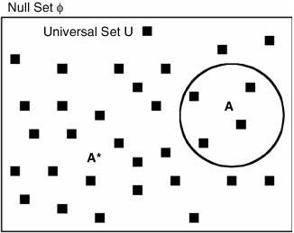
   Total probability

   Probability of event A or event B or both a "success:"

   

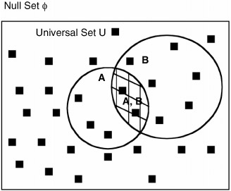
   P(A + B)	‰	P(A) + P(B) - P(A · B)
   	=	1 - P(A* ·B*)
   	=	1 - P(A*) · P(B*), if independent

   Probability of not A "AND" not B: (where not A = A*)

   P(A* · B*) = 1 - P(A + B)

3. Series system of events

   1. No redundancy (A chain is as strong as its weakest link.)

   Product rule for individual independent probabilities (Series components):

   

   Joint Probability:

   • P(A ‹‚ B) = P(A · B)

   

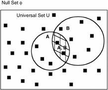
   P(A · B)	=	(A)P(B A)
   	=	P(A)P(B), if independent

   Note  

   1. Independent is not the same as "mutually exclusive."

   2. Individual probabilities are always less than unit.

   3. Product probability for the series is always smaller than lowest individual series components.

   NUMERICAL EXAMPLE

   Components A and B represent events both of which must be satisfied simultaneously for system function. Past history indicates that the individual probability of these components to function properly is:

   P(A) = 0.90 and P(B) = 0.80

   The probability that the system will function properly is then the probability of component A "AND" the probability of component B.

   Since A and B are assumed to be independent events, the probability of the series is

   P(A · B)	=	(A)P(B A)
   	=	P(A)P(B)
   	=	0.9 · 0.8
   	=	0.72

   In any series system,

   The probability of the series system is less than those of either of the individual components.

   In the series configuration, if any of the components fail the entire system fails.

   2. Series components

      

      A system consists of a series of n components (no redundancy).

      Successful operation of each component is independent (independent implies components do not interact).

      Reliability of individual components:

      R _i = P(A _i ) = p _i

      Unreliability of individual components:

      Q _i = P(A* _i ) = 1 - p _i = q _i

      System reliability is the joint probability of all components:

      

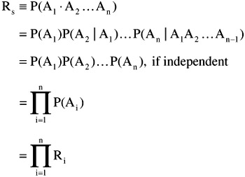
      Note  

      Serial system reliability is product of individual reliability of the components R _i . Series systems are inherently less reliable.

      System unreliability:

      
    

   A system consists of a series of three identical switches.

   Assume 1: Each switch has the same probability not to fail of p.

   Assume 2: Performance probability of each switch is independent.

   System reliability: Probability of system not failing

   R s	‰	P(A 1 , A 2 , A 3 )
   	=	P(A 1 )P(A 2 A 1 )P(A 3 A 1 A 2 )
   	=	P(A 1 )P(A 2 )P(A 3 ), if no interaction
   	=	p · p · p = p 3

   System unreliability: Q _s = 1 - R _s = 1 - p ³

    

   NUMERICAL EXAMPLE

   Assume each switch has a reliability or probability of "successful" performance of 90%.

   P(A _i ) = R _i = p = 0.90

   System Reliability: R _s = 0.90 · 0.90 · 0.90 = 0.729

   Unreliability of individual switch: Q _i = 1 - R _i = 0.10

   System unreliability:

   Q _s = 1 - R _s = 1 - p ³ = 1 - (0.90) ³ = 1 - 0.729 = 0.271

    

4. Parallel system of events ” some form of redundancy

   Total or cumulative rule for individual independent probabilities:

   

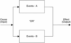
   Total Probability:

   • P(A ‹ƒ B) = P(A + B)

   

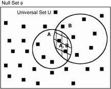
   P(A + B)	‰	P(A) + P(B) - P(A · B)
   	=	P(A) + P(B) - P(A)P(B A)
   	=	P(A) + P(B) - P(A) · P(B), if independent

   Note  

   1. Individual probabilities are always less than unity.

   2. Because of redundancy, total probability for the parallel system can be greater than the smallest component.

   NUMERICAL EXAMPLE

   Components A and B represent events both of which must be satisfied simultaneously for a system function. Past history indicates that the individual probability of these components to function properly is:

   P(A) = 0.90 and P(B) = 0.80

   The probability of the system to function properly is then the probability of component A "OR" the probability of component B.

   Since A and B are assumed to be independent events, the probability of the parallel system is:

   P(A + B)	‰	P(A) + P(B) - P(A · B)
   	=	P(A) + P(B) - P(A) · P(B)
   	=	0.90 + 0.80 - 0.90 · 0.80
   	=	1.70 - 0.72
   	=	0.98

   The reader should notice that the redundancy of the parallel system that allows either-or components to function results in a system that remains functional with higher probability than the probability of either of the individual components acting alone. Therefore, redundancy increases reliability, which means that a system of n components is connected in parallel. Another way of looking at this is:

   1. Successful operation of each component is independent. Again, independent here implies components do not interact.

   2. Each component has a reliability P(A _i ) = p _i ; failure probability of each component is P(A* _i ) = Q _i = 1 - p _i = q _i

   Pictorially this may be shown in Figure 14.1.

   
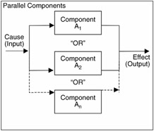
   Figure 14.1: Parallel components.

   We can see then from Figure 14.1 that the System Reliability is the total probability of all components. This also may be shown as:

   

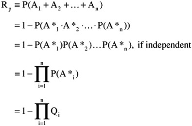
   System unreliability:

   
    

   GENERAL EXAMPLE A

   In the previous example, we had: P(A) = 0.90 and P(B) = 0.80. If this is a parallel system then

   R _p =1 - P(A*)P(B*) = 1 - 0.10 0.20 = 1 - 0.02 = 0.98

    

   GENERAL EXAMPLE B

   A system consists of 3 identical switches in parallel.

   Assume 1: Each switch has the same probability not to fail of p.

   Assume 2: Performance probability of each switch is independent.

   System Reliability: Probability of system not failing: (q = 1 - p)

   R p	‰	P(A 1 + A 2 + A 3 )
   	=	1 - P(A* 1 A* 2 A* 3 )
   	=	1 - q · q · q = 1 - q 3

   System Unreliability: Q _p = 1 - R _p = 1 - (1 - q ³ ) = q ³

    

   NUMERICAL EXAMPLE

   Assume each switch has a reliability or probability of "successful" performance of 90%, which corresponds to 10% "failure."

   Individual Switch Reliability: P(A _i ) = R _i = p = 0.90

   Individual Switch Unreliability: P(A* _i ) = Q _i = q = 0.10

   System Reliability: R _p = 1 - 0.1 · 0.1 · 0.1 = 1 - 0.001 = 0.999

   System Unreliability: Q _p = 1 - R _p = q ³ = (0.1) ³ = 0.001

    

   Example 1: SIMPLE COMBINATION OF SERIES-PARALLEL SYSTEM

   

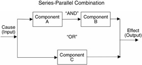
   Probability of success for individual components: P(A), etc.

   Probability of failure for individual components: P(A*), etc.

   Probability of success in series branch ("AND") if independent:

   P(AB) = P(A)P(B) = 1 - P(A* + B*)

   Reliability is success probability of series-parallel system shown:

   R sys	‰	P(AB + C) = P(AB) + P(C) - P(AB)P(C)
   	=	P(AB)[1 - P(C)] + P(C)
   	=	{1 - P(A * + B*)}[P(C*)] + P(C)
   	=	P(C*) - P(A * + B*)P(C*) + P(C)
   	=	P(C*) + P(C) - P(A * + B*)P(C*)
   	=	1 - P(A* + B*)P(C*)

   If probability of all components equal: P(A) = P(B) = P(C)= p

   R _sys = 1 - (1 - p ² )(1 - p) = 1 - q ³

    

   Example 2: SIMPLE COMBINATION OF PARALLEL-SERIES SYSTEM

   

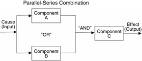
   Probability of success for individual components: P(A), etc.

   Probability of failure for individual components: P(A*), etc.

   Probability of success in parallel circuit ("OR") if independent:

   P(A + B) = P(A) + P(B) - P(A)P(B)

   Reliability is success probability of parallel-series system shown:

   R sys	‰	P([A + B]C) = P(A + B)P(C)
   	=	[1 - P(A*B*)]P(C)
   	=	[1 - P(A*)P(B*)]P(C)
   	=	1 - [1 - P(A)(1 - P(B))]P(C)

   If probability of all components equal: P(A) = P(B) = P(C) = p

   R _sys = [1 - 1 - p ² ]p = [2p - p ² ]p = [1 - q ² ]p

    

   Example 3: SIMPLE COMBINATION OF PARALLEL-SERIES SYSTEM

   

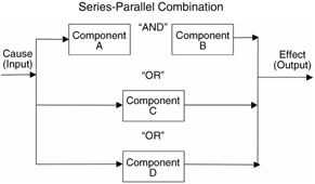
   Reliability is success probability of series-parallel system shown:

   R _sys = P(AB + (C + D)) = P(AB) + P(C + D) - P(AB)P(C + D)

   Joint and total probabilities can be expressed in term of individual probabilities.

   Series branch has joint probability: P(AB) = P(A)P(B)

   Parallel branches have total probability:

   P(C + D) = P(C) + P(D) - P(C)P(D)

   If probability of all components equal: P(A) = P(B) = P(C) = P(D) = p

   R _sys = p ² + p + p - p ² - p ² (p +p - p ² ) = 2p - 2q ³ + p ⁴

    

   Example 4: SIMPLE COMBINATION OF PARALLEL-SERIES SYSTEM

   

   Reliability is success probability of series-parallel system shown:

   R sys	‰	P[D · (AB + C)]
   	=	P(D)P[(AB) + C]
   	=	P(D)[P(AB) + P(C) - P(AB)P(C)]
   	=	P(D)[P(A)P(B) + P(C) - P(A)P(B)P(C)]

   Note  

   This form may be more convenient to use than that developed in Example 1 where we introduced the complement probabilities.

   If all probability of all components equal: P(A) = P(B) = P(C) = p

   R _sys = p[p · p + p - p · p · p] = p ³ + p ² - p ⁴

    

5. Sequence tree diagram

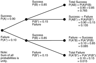
   A tree diagram is very useful in determining decisions where probabilities are known and they are of two options. An example adapted from O'Connor (1996) will illustrate the point. The reliability of missile A to hit target is 90%; that of missile B is 85%.

   A salvo of both missiles is launched. Determine the possibility of at least one hit.

   The tree diagram indicates that four mutually exclusive outcomes may occur:

   

   Probability of at least one hit:

   • P(AB) + P(AB*) + P(A*B) = 0.765 + 0.135 + 0.085 = 0.985