Applying the Extended Use Case Test Design Pattern | Succeeding with Use Cases: Working Smart to Deliver Quality

Robert Binder (2000) has laid out a process for defining a suite of test cases for use cases as part of his Extended Use Case Test Design Pattern. There are four steps in the process:

1.	Identify the operational variables of the use case
2.	Define the domain of each variable
3.	Develop an operational relation for the use case
4.	Build test cases

Not to put too fine a line on it, the approach identifies a set of operational variables and an operational relation, which are to use cases what instance/member variables and class invariant are to a class, respectively. The combinations of different operational variable values and relationships between the variables define the various states of the use case, each state corresponding roughly to a different scenario or "variant" of the use case.

In this section, you will see this four-step procedure applied to the chemical tank example from the previous chapter. The description will deviate slightly from Binder's to better fit the model-based specification approach, which includes preconditions, postconditions, invariants, and unprimed/primed state variables.

A key point to gain from this section is that by building a model-based specification, as was done in the previous chapter, you have essentially done all the hard work of test design: a model-based specification is what Binder calls a test-ready model, and all that is left is to essentially "fill in the blanks" of the Extended Use Case Test Design Pattern.

Step 1. Identify Operational Variables

Binder's procedure begins by identifying the operational variables: those factors that vary from scenario to scenario and which determine different results from one use case scenario to the next.^[2] Operational variables include inputs, outputs, and abstractions of the state of the system as examples; all items that our model-based specification of the use case supplies. The operational variables for the chemical tank use case are the initial state variables (unprimed), outputs, and changed state variables (primed) utilized in the model-based specification of the use case:

^[2] Binder actually says different "variants" and makes a distinction between variants and scenarios; for simplicity, the focus here will be scenarios.

InFlow Initial rate of flow into the tank when the use case starts.
OutFlow Initial rate of flow out of the tank when the use case starts.
Delta The incremental increase in rate of flow into the tank used for refilling: A constant whose actual value the model does not specify.
InFlow' The flow rate to increase the level in the tank.
InFlow" The flow rate at the end of the use case to stabilize the level.
OutFlow' The rate of flow out of tank subsequent to the start of refilling through to the end of the use case.

This is a good opportunity to re-emphasize that primed and unprimed versions of a variable are actually separate variables in the model. InFlow, InFlow', and InFlow" are separate variables representing three separate states of one aspect of the chemical tank, that is to say the rate of flow into the tank. If they were not separate variables in the model, one would not be able to specify relationships between them (e.g., InFlow" < InFlow').

Independent Operational Variables

Having identified the set of operational variables, it remains to identify which are independent: an independent variable is one that is not defined in terms of another variable and therefore can be varied for testing purposes. In a model-based specification, these are generally inputs (parameters passed into the use case, which we do not have in our chemical tank example) and the initial, unprimed state variables. For our example, the independent variables are:

InFlow initial rate of flow into the tank when the use case starts
OutFlow initial rate of flow out of the tank when the use case starts
OutFlow' the rate of flow out of tank subsequent to the start of refilling through to the end of the use case

It is not common to have a primed variable, such as OutFlow', as an independent variable in a model-based specification, but in this case, this variable is not defined in terms of other variables, is controlled external to the use case by the rate of production of manufacturing, and so can be manipulated for testing purposes.

Step 2. Define Domains of the Operational Variables

The second step of the Extended Use Case Test Design Pattern is to define the domain of each operational variable: the set of all possible values. As part of the model developed in the last chapter, these domain definitions have already been defined:

0 InFlow MaxFlow
OutFlow MaxFlow

Recall that MaxFlow is some upper bound that specifies the maximum safe rate of flow into, or out of, the chemical tank. It is a positive constant whose specific value is not addressed in the model.

Because domain definitions are essentially global data invariants, the following are also true:^[3]

^[3] This concept was discussed in Chapter 5, "Preconditions, Postconditions, and Invariants: What They Didn't Tell You, But You Need to Know!" Refer to the "Global Invariants: Preconditions on Steroids" section.

0 InFlow MaxFlow
InFlow MaxFlow
OutFlow MaxFlow

Step 3. Develop the Operational Relation

Relations are a common way to specify the expected behaviorand hence test casesof all manner of "black boxes," be they software or hardware. They allow us to specify what something should do without having to say how it is to be done. The Extended Use Case Test Design pattern applies this idea to use cases in the form of what is called an operational relation, implemented via a decision table.^[4] In this step, we'll take the preconditions, postconditions, and invariants of our model-based specification and put them into the decision table format of Binder's Extended Use Case Test Design Pattern.

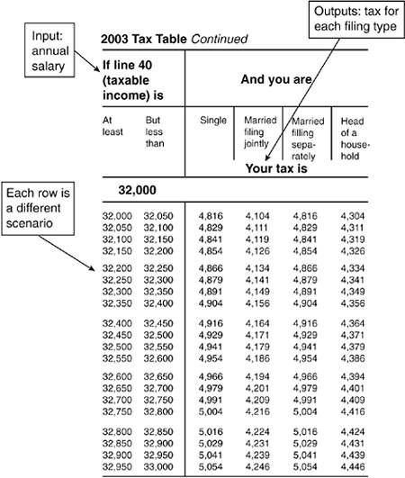
^[4] Leffingwell and Widrig (2003) use a similar approach to specify test cases but call it a matrix.

Tables as Relations

A common way to think of a relation is as a table. Figure 6.1 is part of a table for computing personal income tax in the United States.

Figure 6.1. Table for computing personal income tax in the United States.

The tax table in Figure 6.1 defines a relationship between an inputyour annual taxable income (line 40 on the tax form)and various outputs, taxes due, for various filing status: single, married filed jointly, married filing separately, and head of household. Each row provides a different scenario in your own personal "paying taxes" use case; if your income meets the conditions predicated on the inputs (your income is "At least" X "But less than" Y), that row outputs the tax rates that apply to you for the various filing statuses. If you were testing a software program for doing personal income taxes, you might use a table such as this to specify the expected outputs of the program.

Operational Relation Table for Chemical Tank Use Case

Binder's operational relation applies this use of relations, implemented via a decision table, to specify the expected behavior of use cases. To implement the operational relation, one needs to specify the relationships that exist between each of the operational variables. We begin by listing the operational variables as columns in a table, as shown in Figure 6.2.

Figure 6.2. Operational variables form the columns of the operational relation of the chemical tank use case.

The first three columns are the independent variables that can be controlled for testing. The next four columns provide the expected results: outputs and state change that we expect to see. An extra column (last) has been added to the model to output status messages.

Next, we populate the first row with the use case main scenario, using the domain definitions, preconditions, postconditions, and invariants from our model-based specification to specify the range of values of each operational variable, constraints on, and relationships between, the operational variables (see Figure 6.3).

Figure 6.3. Operational relation for main scenario of the chemical tank use case.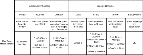

In Binder's operational relation, one scenario of the use case is allocated one row of the table. Because our use case for refilling the chemical tank only has a main scenario, the table has just one row. Keep in mind, however, that this one row is like a database query: it uses variables to describe all possible instances of the main scenario.^[5]

^[5] In set theory, relationswhich are sets of "records," to use a database analogycan be described in two ways: by extension, like the tax table in Figure 6.1, where every record of the relation is enumerated one by one; or by intension, like the operational relation in Figure 6.3, where variables are used to describe the properties of all records of the relation, just like a database query. They are both relations, just described in different ways. This distinction is also called set enumeration versus set comprehension.

That's it; the operational relation is defined. As this example illustrates, a model-based specification with its preconditions, postconditions, and invariants is itself a description of a relation,^[6] so it is just a matter of rearranging the information to put it into the format of the Extended Use Case Test Design Pattern's operational relation.

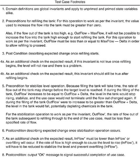
^[6] Model-based specification is rooted in set theory, of which relations are a part.

An Alternate Format for the Operational Relation Table

As just noted, in Binder's operational relation, one scenario of the use case is allocated one row of the table. While this results in a compact table, there are drawbacks. First, use cases are by their nature workflow oriented, often describing step-by-step procedures. This workflow information can be useful for testers during testing. Placing a scenario in one column tends to compress out this workflow aspect of the use case; information that might be useful to testers is lost. Second, restricting a scenario to a single row also makes it difficult to see which preconditions, postconditions, and invariants are working together as a team.

To address these two issues, you may find this alternate, expanded format useful in which each use case scenario gets its own table (see Figures 6.4 and 6.5).

Figure 6.4. Operational relation with main scenario in expanded format (each scenario gets its own table). Gray shows preconditions, postconditions, and invariants that are working together to describe a use case step.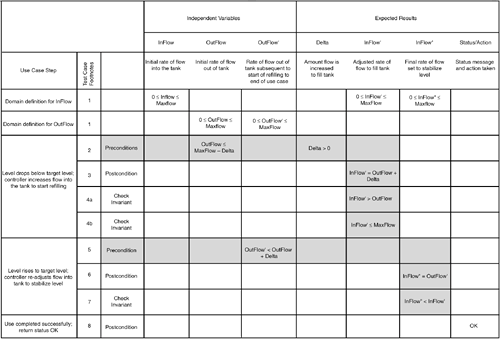

Figure 6.5. Test case footnotes for the operational relation of Figure 6.4.

This expanded format has a number of advantages. First, the workflow nature of the use case is preserved: use case stepsstated in natural languageare listed in the first column. The second column allows references to footnotes that are pertinent to testing; footnotes are listed at the bottom of the table (refer to Figure 6.5).

Second, this overall combination of natural language augmented with a model provides a test case that is both understandable while also being rigorous. Al Davis' (1995) philosophy on requirements"Augment, Never Replace, Natural Language"is, I believe, as appropriate for test cases as it is for requirements.^[7]

^[7] See (Davis 1995), particularly Principle 54: Augment, Never Replace, Natural Language.

And finally, the team of preconditions, postconditions, and invariants that models and describes a use case step is directly associated with the step, and each item receives a row in the matrix.^[8] The team that plays together stays together!

^[8] An alternate approach is to allocate each use case step one row and combine all its associated preconditions, postconditions, and invariants on that one row.

It's worth re-emphasizing that the content of Figure 6.4 is the same as that of Figure 6.3: if the former were collapsed into a single row it would result in the latter.

Step 4. Build Test Cases

The final step of the Extended Use Case Test Design Pattern actually involves two tasks:

The selection of test points: values to be used for inputs and state variables in test cases. The Extended Use Case Test Design Pattern calls for two types of test points:

a. Valid test points: for a model-based specification, this involves test points where all preconditions and invariants are satisfied.

b. Test points that should cause a failure: for a model-based specification, this involves test points where at least one precondition/invariant fails. This is essentially a test of the software's error-handling capability.

The creation of test cases using the selected test points.

The next two sections look at these tasks in more detail.

Select Test Points

In our operational relation of Figure 6.4, we have three independent variables for which we need to select test points: InFlow, OutFlow, and OutFlow'. Remember, the independent operational variables are the ones not defined in terms of other operational variables, so they are the source of variation for testing purposes.

As noted previously, preconditions are a good source from which to select test points for an independent variable. But a variable may be constrained by several preconditions in a use case scenario: the valid test points we identify must simultaneously satisfy all preconditions that constrain a variable as well as its domain definition.^[9] Figure 6.6 illustrates a straightforward, low-tech approach you can use to identify such test points.

^[9] In software testing, the process of selecting test points from an input's or state variable's domain by analyzing constraints on the variable is called domain analysis (Binder 2000).

Figure 6.6. Valid test points for a variable must satisfy its domain definition and all preconditions in the use case that constrain it.

In the table in Figure 6.6, the independent operational variables for the use case are listed across the top as columns. The domain definition (the set of all possible values) for each variable is listed in the first row of the table (refer to section "Step 2. Define Domains of the Operational Variables"). In subsequent rows, any preconditions that further constrain the values of each variable are listed. Finally, for each variable the final row shows the subset of the domaincalled a subdomainthat meets all the preconditions in a column. This is arrived at by simple visual inspection looking for the "lowest common denominator" for each column, so to speak. That subset, or subdomain, is then entered in the last row of the column.^[10]

^[10] Rather than building a separate table, in "real life" you might do this directly from inspection of the operational relation itself as it is the source of domain definition and preconditions for the table. The table in Figure 6.6 is constructed here primarily as an aid to the reader, helping to focus on just the parts of the operational relation that are pertinent.

It is the last row of the table in Figure 6.6 from which test points for InFlow, OutFlow, and OutFlow' should be selected. The table in Figure 6.7 shows test points (rows) to be used for valid and failure scenario test cases selected from each variable's subdomain (columns).

Figure 6.7. For the upper and lower boundary of each variable's subdomain, two test points are selected: one that is valid and one that should cause a failure. Flow rates are stated in Gallons Per Minute (gpm).

The test points of the table in Figure 6.7 were selected using the "1xx1" or "one-by-one" domain testing strategy.^[11] For the variables of Figure 6.7, each subdomain has two boundaries: a lower bound and upper bound. The one-by-one strategy calls for two test points per boundary: one that is valid and one that should cause failure. For the example here this results in a total of four test points per variable.

^[11] The Extended Use Case Test Design Pattern does not suggest a particular test point selection strategy other than that test points should include valid test points and test points that should cause failure. The one-by-one strategy certainly meets this criterion. See Binder (2000), particularly the "The One-By-One Selection Criteria" section.

Test points having been selected, they now need to be incorporated into test cases.

Use Test Points in Test Cases

The final task of the Extended Use Case Test Design Pattern is to use the test points of Figure 6.7 in actual test cases, including expected results. Expected results for valid test points can be determined using the operational relation of Figure 6.3 or Figure 6.4.

For test points intended to cause failure, the operational relation would need to be extended to cover each failure scenario. For the sake of brevity, such an extension is not shown here, although it is assumed such an extension is available as a basis for determining the expected results of the failure test points.

While valid test points can be combined into the same test case, test points intended to cause failure typically require a test case of their own. Hence, as is clear from the table in Figure 6.7, the chemical tank use case requires six different test cases to cover each of the six failure scenarios identified. Briefly, the failure scenarios are as follows:

Failure Scenario 1 Backwash in the InFlow valve when use case starts (i.e., InFlow is negative)
Failure Scenario 2 Initial InFlow is too high at start of use case
Failure Scenario 3 Backwash in the OutFlow valve when use case starts (i.e., OutFlow is negative)
Failure Scenario 4 Initial OutFlow at start of use case is so high that tank can't be refilled at rate Delta without raising InFlow' past the MaxFlow rate
Failure Scenario 5 OutFlow' is set to be negative (backwash) after refilling begins but before target level is reached
Failure Scenario 6 OutFlow' is increased to be OutFlow + Delta after refilling begins but before target level is reached

Figure 6.8 shows a table of test cases in the style of the Extended Use Case Test Design Pattern with one test case per row. Shown are two valid tests of the main scenario and six failure scenario tests. Blank cells indicate that the value of the corresponding variable is irrelevant; Binder uses "DC" (Don't Care) for this purpose. Footnotes (none shown) would provide additional explanation to the tester on test setup, execution, and expected results, including preconditions and invariants to be aware of and/or monitored.

Figure 6.8. Table of test cases in the style of the Extended Use Case Test Design Pattern.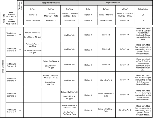

With test cases in place, the Extended Use Case Test Design Pattern is complete.