Oracle Data Mining

9.2 Oracle Data Mining

Data mining is a process that finds hidden patterns and relationships in data to help you make better business decisions.

In the course of running a business, you may encounter data in different forms. Operational data tells you day-to-day information about your customers—what did John Doe buy on August 5, 2002? In the data warehouse, data is organized according to predefined relationships using fact and dimension tables. You can then use OLAP tools to find out various facts about your business. How many people bought electronic products from your store and what was the average amount they spent? How many customers who bought electronic products were engineers? These are all questions based on existing data.

However, you may also like answers to questions such as:

• Which of your customers are likely to buy a personal video recorder?

• What could be a good city to launch a new product?

• What might be a good promotion to offer for Christmas?

This is where you need some predictive insight into your data. Data mining uses various statistical and machine learning techniques to discover trends and patterns of behavior. In some cases, you may know what you are looking for. In other cases, there is no clear definition of what the mining process may find. You are saying: Here is my data—go find me something interesting to look at. This is indeed the challenge of data mining—it is like finding a needle in a haystack, only you may not know what the needle looks like! One of the biggest advantages of building a data warehouse is that data has been cleansed and consolidated and is now more amenable to data mining.

Data mining can be used in many applications, such as improving store layouts, fraud detection, mail-order promotions, reducing customer churn, and Web site personalization. It can also be used in life-sciences applications, such as finding patients at high risk for certain diseases.

Oracle 9i data mining option

Oracle data mining is an option to Oracle 9i Enterprise Edition that embeds data mining functionality in the server. Data mining involves processing large amounts of data. The data often needs to be preprocessed and put into a format suitable for the mining algorithms. By incorporating mining functionality into the database, the mining algorithms can take advantage of Oracle's scalability and features such as partitioning, compression, and parallel execution to speed up the analysis.

Oracle data mining is a Java API that supports association rules, classification, and clustering. Oracle is the lead sponsor of the Java Data Mining (JSR-73) Specification for data mining. Over future releases, Oracle data mining will conform to this standard once Java data mining attains reference status.

Oracle data mining should not be confused with Darwin, also known as Oracle Data Mining Suite. This product did the data mining analysis outside the database and has now been discontinued. Darwin had a graphical interface with point-and-click capability, but it was extremely difficult, if not impossible, to integrate data mining directly into your applications with this product. On the other hand, Oracle data mining allows you to embed data mining directly into your application logic and workflow, rather than extracting data out of your applications for analysis.

Unlike much of the other material in this book, data mining algorithms need some mathematical background, such as statistics and probability. In this section, we will provide you with a broad overview of the data mining process and techniques while avoiding the technical details of each algorithm. We will describe the tasks and briefly illustrate the use of Oracle Data Mining Java API. To read the examples at the end of this chapter, you must have a basic knowledge of the Java programming language. However, if you are only looking for a conceptual overview, you may safely skip these examples.

9.2.1 Oracle data mining techniques

Data mining problems can be classified into two categories. In some situations you have some idea of what you are looking for—for example, you are interested in customers who are likely to buy a digital camera. This is known as directed or supervised learning. In other cases, you leave it to the mining process to find you something interesting—for example, a high incidence of accidents at a certain intersection. This is called undirected or unsupervised learning.

Oracle data mining supports various techniques for mining data, each of which falls into one of these two categories.

• Association (undirected)

• Clustering (undirected)

• Classification (directed)

We will look at each of these in some detail.

Association rules

You are probably familiar with Amazon.com's feature: Hello Jane! We have some new recommendations for you. This type of Web site personalization uses a data mining technique known as association rules. Mining with association rules finds items that occur together frequently. For instance, it may find that a large percentage of users who bought the book The Lord of the Rings also bought the book The Hobbit. So if you buy The Lord of the Rings, it may recommend you also read The Hobbit.

Data mining using association rules is also known as market-basket analysis. When you visit your local grocery store, you may find that the seafood department has lemons or tartar sauce next to the fish. This is because they may have found that 80 percent of people who buy fish also buy lemons to go with it. Most of these stores offer some kind of frequent shopper cards—by keeping a count of what combinations of items have been bought by the same person, they can organize their shelves more appropriately and even send you coupons for the same or similar items for your next visit.

Mining with association rules involves counting how many times a certain group of items occur together. In this case, you do not necessarily know what combination to look for—hence, this comes under the unsupervised or undirected learning category. The association algorithm comes up with rules of the type "A implies B." There are two quantities of interest to the user of this algorithm—support and confidence.

• Support tells us the percentage of the transactions where the combination of items A and B occur together. It helps identify combinations that are sufficiently frequent (e.g., purchasing fish or purchasing fish and lemons).

• Confidence tells us what percent of transactions that have an item A also have an item B (e.g., how many transactions that have fish also have lemons).

To use association rules, a user must provide the desired level of support and confidence for a rule to be considered interesting. For instance, suppose we specify a support of 20 percent and confidence of 70 percent. If we found that 50 percent of all transactions involve fish and 40 percent of all transactions involved the combination fish and lemons, then the combination "fish, lemons" is interesting because it exceeds the minimum support of 20 percent. In this example, the combination "fish, lemons" has confidence (40/50) * 100 = 80%, so it also meets the minimum confidence criterion. Hence, "fish implies lemon" will be reported as an association rule.

To make meaningful business decisions, both support and confidence are important. Consider this alternate example of an area where fish is not very popular due to high levels of mercury. Maybe only 5 percent of the transactions involve fish. The item "fish" does not have enough support, and hence the rule "fish implies lemons" will not make any significant difference to our sales.

Figure 9.36 shows a typical output of mining analysis using association rules, as analyzed using Oracle 9i Discoverer. The first two rules say people often buy wine or lemons to go with fish.

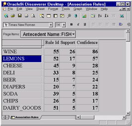
Figure 9.36: Association rules.

Clustering

Clustering is a technique used to divide a large data set with many attributes into a small number of closely packed groups. Such groups are not easily apparent to a human eye due to the large number of attributes involved. For example, suppose you had census data for a population, including several attributes such as age, occupation, occurrence of diseases, and so on. By clustering this data, you may find that there are several pockets where a certain disease is prevalent, possibly pointing to a polluted water supply in those regions. Since we have no definite idea of what we may find, this is another example of unsupervised learning.

The groups generated by a good clustering algorithm are such that all items in one group are quite alike each other in some respect and very much unlike items in other groups. Figure 9.37 illustrates the concept of clusters in data. In this figure, two attributes of the data has been plotted using a scatter plot to highlight the clusters. For all items in each cluster, the values of the two attributes have greater similarity compared with items in different clusters. This is an example where the clusters in the data were apparent by simply plotting a graph. In practice, it is not often possible to visualize clusters in this way, since we may have more than two or three dimensions! For instance, in bioinformatics applications, you can have thousands of dimensions! In these situations, we use mathematical clustering algorithms to identify clusters.

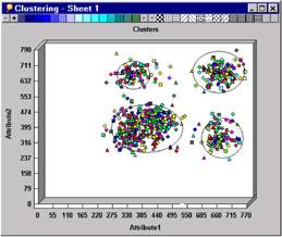
Figure 9.37: Clustering.

One of the applications where clustering is used is market segmentation. Suppose you were a large retailer selling a wide range of products from soaps to jukeboxes. With clustering, you can segment your customer base into groups based on demographics or past buying habits. This allows you to customize your advertising strategy for each segment and to better serve the more profitable segments.

Clustering is performed by first analyzing a small section of the data to determine clusters. Once the clusters have been determined, the remaining data is then analyzed to assign each individual item to a cluster, with a certain probability.

Classification

Suppose you wanted to target a promotion for a new digital camera and would like to know which of your customers are likely to buy the camera. Classification is a data mining technique that is useful for this application. Classification divides data into two or more well-defined classes. Unlike clustering, where you do not know what groups will be generated, in classification you know exactly what each group represents. In the previous example, the two groups are customers who are likely to buy a camera and customers who are not likely to buy the camera. This is an example of supervised learning.

In classification, you first analyze a small part of your data to build a model. For instance, you would analyze real data for people who have bought digital cameras over a given time period. The data used to build a model is known as build data. The model will be built taking into account various factors, such as age, income, and occupation, that are known to influence people's buying habits. These factors are known as predictor attributes. The output that is predicted is called the target attribute, and its values (whether the person will buy the camera or not) are known as categories or classes. Once the model has been generated, it can be applied to other data to come up with a prediction. This is known as model apply or scoring. In our example, you would use the model to predict if a certain customer is likely to buy a digital camera.

In this example, the target attribute has two values—will buy a digital camera and will not buy a digital camera. You can also use classification to predict attributes with more than two values—for example, whether the risk of a person defaulting on a payment is low, medium, or high.

Classification is often used to create customer profiles. For instance, once you have determined which of your customers are likely to buy a digital camera, you can then profile them by occupation, as shown in Figure 9.38. From this graph, you can see that most likely buyers are either engineers or executives. So you can now target your promotions more accurately toward these customers and reduce your costs.

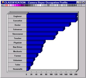
Figure 9.38: Classification.

In order for classification to work well, the build data must contain enough samples for each target category; otherwise, the results may not be accurate. In other words, your build data must include enough people who have bought digital cameras in the past and enough who have not.

Testing a classification model

Data mining using classification usually involves a testing phase to check how good the model is. For this, data where the outcome is known is tested to see how well the model's predictions match the outcome. For instance, you could take data for customers who have bought a digital camera in the past and check this data against the predictions given by the model.

Testing a model involves computation of a structure known as the confusion matrix. A confusion matrix tells you how many times the model's prediction matched the actual data and how many times it did not. The columns correspond to the predicted values and the rows to the actual values. For instance, in Figure 9.39, the model was correct 555 + 45 = 600 times and wrong 12 + 8 = 20 times. This shows that this model is a pretty good one.

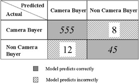
Figure 9.39: Confusion matrix.

Computing Lift

Another metric used to determine the effectiveness of a model, is its lift. To understand what lift means, consider the following example. Suppose we have a customer base of 100,000 households and on an average about 2.5 percent (2,500 customers) respond to any given promotion. We would like to get smarter and only target those customers who are most likely to respond. With a good classification model, we should be able to identify most of the likely 2,500 respondents by targeting much fewer than the 100,000 households. Given a certain percentage of target customers, lift is the ratio of the number of respondents obtained with the model against the number obtained without the model.

Lift is computed as follows. The classification model is applied to an actual customer data set where we know who responded to a past promotion and who did not. The customers are then sorted by their likelihood to respond as predicted by the model, with the most likely respondents first. This sorted list is then divided into ten equal groups known as deciles. For each decile, the number of customers in the data set that had actually responded to the promotion is counted. If the model is any good, most of the respondents should come from the top few deciles, since they were predicted to be the most likely respondents.

If you draw a graph with deciles one through ten on the X-axis and the number of actual respondents on the Y-axis, you will typically get the curve as shown in Figure 9.40. This curve tells you that you only need to target the customers in the first three deciles (30 percent of households) to get 70 percent of those likely to respond. On the other hand, the straight line in this figure corresponds to a random promotion, where everyone is predicted to be equally likely to respond. Without the model to guide you, if you target 30 percent of households, you will only get 30 percent of the likely respondents. To get 70 percent of the likely respondents, you will have to target 70 percent of households! The higher the curved line is from the straight line for the first one or two deciles, the better the model's lift.

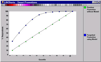
Figure 9.40: Using lift analysis for targeted promotions.

Confusion matrix and lift are both widely employed techniques to determine the accuracy of classification models. Oracle data mining provides APIs that will allow you compute these quantities.

9.2.2 Oracle data mining algorithms

Now that we have seen the techniques that are used in data mining, we will briefly look at the various algorithms offered by Oracle for each of these techniques.

Association rules

The algorithm used by Oracle data mining for association rules is called Apriori. The user provides the minimum support and confidence desired. The algorithm first finds single items that occur frequently and have the minimum support—for example, fish. It then finds pairs of items that have the minimum support such that at least one item in the pair was itself frequently occurring—for example, fish and lemons. It repeats the process to come up with increasingly larger combinations of items until it can find no more. Once it has found all frequent item sets, it finds those among them that satisfy the minimum confidence requirement from the user. These are reported as association rules.

Classification

Oracle offers two main algorithms for classification: Naïve Bayes algorithm and Adaptive Bayes Network algorithm.

The Naïve Bayes (NB) algorithm is based on a probability theorem known as Bayes theorem and assumes that each attribute is independent from the other. An interesting property of the NB algorithm is that you can build and cross-validate the model using the same data. This algorithm works best with a small number of predictor attributes (less than 200).

The Adaptive Bayes Network (ABN) algorithm produces a model in the form of a decision tree, such as that shown in Figure 9.41. From this decision tree you can see that men between the ages of 15 and 35 and women over 26 are likely to buy a camera. Since the model produced by ABN is in a human-readable form, a business analyst or executive would be more comfortable when using it to make a business decision. The ABN algorithm is also more accurate than NB, but it takes longer to build the model.

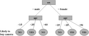
Figure 9.41: Adaptive Bayes Network decision tree.

In addition, Oracle also offers a Model Seeker feature. This feature allows you to generate multiple models using the ABN or NB algorithms and then determines which is the best with regards to a specific target category. For instance, it could tell you which model best predicts people who may buy a digital camera, or which model best predicts people who will buy kitchen appliances. Model Seeker also generates a summary of all the models it built so that the user can determine which model is the best.

Clustering

Oracle data mining supports two algorithms for clustering: Enhanced k-means and O-Cluster.

The k-means algorithm is a clustering algorithm that groups data into a specified number of k clusters. It groups items into clusters based on their relative distance from each other. So, all points in one cluster are closer to each other than to points in other clusters. The Enhanced k-means algorithm is a variation on the k-means algorithm, which forms clusters in a hierarchical fashion. It starts with all the data being in one cluster and then successively splits this data into smaller clusters until the desired number of clusters is obtained. It is very efficient compared with traditional k-means, since it only requires one pass through the data and hence can handle large data sets. It works well even for data sets with less than ten attributes. The metric distance used by k-means can only be defined for numerical attributes; hence, if you have discrete values (e.g., color = red, black, blue), k-means cannot be used.

The O-Cluster algorithm defines clusters using ranges of attribute values. The user does not need to provide the number of clusters to generate. This algorithm can be used for nonnumeric attributes that have a discrete set of values.

9.2.3 Data preparation in Oracle data mining

In order to use data mining, you may need to preprocess the data to reduce its size or complexity. Binning and attribute importance are two techniques commonly used.

Binning

Data mining algorithms typically require that the data be "binned" into a discrete set of buckets for analysis. Oracle provides the capability to automatically perform binning or allows a user to manually bin the data by specifying the boundary values for the buckets.

Attribute importance

If your data has a large number of predictor attributes, it can be a challenge to determine which ones influence your required target attribute and which ones do not. For instance, age may determine a customer's preference in music. The customer's height or the color of his or her eyes may have little impact. Depending on the number of predictor attributes, the classification process can be quite time consuming to compute. Attribute importance is a technique that automatically ranks attributes by how likely they are to influence the target attribute. This helps you narrow down the relevant predictor attributes before building the classification model.

The algorithm for attribute importance in Oracle data mining is known as predictor variance. It takes as input a data set, along with its predictor and target attributes, and ranks the predictor attributes. It finds how the target attribute changes with changes in each predictor attribute (i.e., computes the variance of the target attribute with respect to the predictor attribute). If the variance is high, it means that the predictor attribute has a significant influence on the target attribute and is ranked higher.

9.2.4 The PMML standard

The Predictive Modeling Markup Language is an emerging XML-based standard to define data mining models. PMML provides a vendor-independent method of defining models so that the models can be exchanged between different applications. Thus one application may produce a model, and another may apply the model to a data set. Oracle data mining supports import and export of association rules and Naïve Bayes models.

9.2.5 Using Oracle data mining

Oracle Data Mining consists of two components: Oracle Mining Server and Oracle data mining Java API.

Oracle Mining Server is a component within the Oracle database that performs the mining tasks. The Mining Server consists of a repository, which stores the tables containing inputs and outputs of the analysis.

Oracle data mining API is a Java API, which allows an application developer to write data mining programs for the techniques discussed earlier.

Installation and configuration

Oracle data mining (ODM) is available as part of the Oracle 9i installation using the Universal Installer. During installation, if you choose to create a preconfigured database (see Chapter 2), ODM is automatically installed for you. You must, however, unlock the ODM and ODM_MTR accounts that came with the preconfigured database and set new passwords, as follows:

 alter user odm identified by <odm_password_here> account unlock; alter user odm_mtr identified bu <odm_password_here> account unlock; 

If you have chosen to build a custom database, you must use the Database Configuration Assistant (DBCA) to install the ODM option and follow its instructions.

It is recommended that you use partitioning (if available) and parallel execution for data mining tasks, especially for large data sets, since they offer significant performance gains.

To use data mining functionality, the ODM Task Monitor must be running. To start the ODM Monitor, log in as the ODM user and issue the following command in SQL*Plus:

 execute ODM_START_MONITOR; 

To stop the monitor, issue the following command:

 execute ODM_STOP_MONITOR; 

Now you are ready to start using the data mining APIs.

Data mining tasks

A typical flow of a data mining analysis will involve the following steps:

1. Preprocessing the input data for analysis: The raw data may need to be preprocessed before analysis. Some algorithms require that the data be binned. The user can preprocess the data and specify how this data is to be binned. This is optional, since Oracle can automatically perform binning, if the user has not done so.

2. Specifying the data to be mined: The data to be mined must be placed in a single table. Each fact in the data being analyzed is known as a case. For example, "customer #3, male, aged 35, a teacher by profession, bought a digital camera" is one case. In the table, a case may be represented using either a single record or multiple records—one for each attribute, as illustrated in Figure 9.42.

   
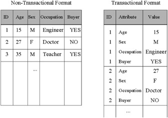
   Figure 9.42: Table formats for data mining.

   If all attributes for a case are placed in the same row, the table is said to be in a nontransactional format. Alternatively, the table could store each case using multiple records with the format (customer#, attribute_name, attribute_value). This is known as a transactional format.

   Regardless of how the data is stored, Oracle will convert the data into a transactional format prior to analysis.

   The input table specification is defined using a Physical Data Specification (PDS) Java object.

3. Setting up parameters for the analysis: Next, you must indicate what function you would like to use (association, clustering, classification, or attribute importance). You can specify parameters at two levels—at the level of the function or technique you want to use and at the level of the actual algorithm you want to use for that technique. If you do not specify the algorithm setting, Oracle will use a default. The function settings for analysis are stored in a Mining Function Settings (MFS) Java object. The actual API to use to create the MFS depends on the mining technique you are using. We will see an example of classification in the next section. An important part of MFS settings is the Logical Data Specification, where you specify how each mining attribute has to be treated by the mining algorithm. This will include the attribute type, as in whether the attribute is categorical or numerical, the use, as in whether it is a target attribute or a predictor, and its preparation status, as in whether the attribute is prepared or unprepared.

   After the mining function settings object is created, it is a good idea to validate it to ensure it is correct. You can also persist the settings object in the database by giving it a name. This allows you to reuse the same settings in different programs.

4. Building a model: Now you are ready to build a model. To build a model, you create a MiningBuildTask object, make it persistent in the database, and then execute it. The model is executed asynchronously. You can query the status of the task during execution. When execution is complete, the model will be stored in the database.

5. Applying the model to new data: Once you have built a model, you can apply it to new data to make predictions. You can apply a model on new cases stored in a table or to a single case. The new data must be preprocessed (if needed) and stored in a table compatible with the one used to build the model. To apply the model, you first describe the location of the new data, as in step 2. Next, you specify the location for the output table where the results or predictions must be placed and identify what subset of attributes should be placed in the output table. Finally, to apply the model, you create a MiningApplyTask object, give it the name of the model you described earlier, and execute it. The results will be stored in the database in the specified output table.

6. Testing a model and computing lift: As described earlier, when using classification you may want to test the model and compute its lift. To test a model and compute its lift, you must specify the location of the test data, which must have the same format as the build data. To test the model create a ClassificationTestTask object and execute it. A confusion matrix is generated and stored in a ClassificationTestResult object. To compute lift, create a Mining-ComputeLiftTask and execute it. The lift values for each decile are stored in a MiningLiftResult object.

Now we will illustrate some of these steps using the Oracle Data Mining APIs.

9.2.6 An example using Oracle data mining APIs

We will present an example of using the APIs for one technique, namely, classification. This will illustrate the general flow of the data mining analysis. (Note: The detailed description of all the APIs is beyond the scope of this book. You can find the entire API specification with your Oracle installation.)

Example 1: Building a model.

We will build a model for classification to predict if a person is likely to buy a digital camera. The input data set is stored in a table, EASYDW.TEST_BUILD_DATA. The data is stored in a nontransactional format, meaning that all attributes for a case are stored in the same row of the table. The table definition is shown in the following code segment. The target attribute, CAMERABUYER, indicates whether the person has bought a digital camera or not. It has the value 1 if the person has bought a digital camera and 0 if not. The example is in the form of snippets of Java code.

 SQL> describe test_build_data;  Name                                    Null?    Type ---------------------------------------- -------- --------------- CUSTOMERID                                        NUMBER(10) AGE                                               NUMBER SEX                                               VARCHAR2(8) OCCUPATION                                        VARCHAR2(10) CAMERABUYER                                       NUMBER(1) 

1. Preprocessing the input data for analysis: We will not pre-process the data and let Oracle automatically perform binning.

2. Specifying the mining server to use: We first create an instance of a DataMiningServer object, specifying the database to connect to using a JDBC URL for the user to log in as. On successful login, we get a connection handle (dmsConn), which will be used in the subsequent APIs.

    DataMiningServer dms = new  DataMiningServer    ("jdbc:oracle:thin:@slawande-pc:1521:orcl",     "odm", "odm"); oracle.dmt.odm.Connection dmsConn = dms.login(); 

3. Specifying the structure of data: We must first create a LocationAccessData object, which indicates the schema and table name of the input data. Then we create a PhysicalDataSpecification object of the NontransactionalDataSpecification type. (If the table were in transactional format, you would use TransactionalDataSpecification instead.)

    LocationAccessData lad = new    LocationAccessData("TEST_BUILD_DATA", "EASYDW"); PhysicalDataSpecification pds = new    NonTransactionalDataSpecification(lad); 

4. Setting up parameters for the analysis: Next, we specify parameters to do classification. We will let Oracle determine the algorithm to use and not specify any algorithm-level settings. The DataPreparationStatus uses a value of "unprepared" to indicate that the data has not been prebinned, and Oracle should apply automatic binning.

   The target attribute is specified as CAMERABUYER and is of type categorical, because it has discrete values.

    ClassificationFunctionSettings cfs  = ClassificationFunctionSettings.create      (dmsConn, null, pds, "camerabuyer",       AttributeType.categorical,       DataPreparationStatus.getInstance         ("unprepared")); 

   If we want to use the Naïve Bayes algorithm, we must also define the algorithm-level settings and pass them into the function-level settings. The code would then look something like the following. Notice that we have passed the Naïve Bayes settings variable nbs into the ClassificationFunctionSettings class.

    NaiveBayesSettings nbs   = new NaiveBayesSettings(0.01f, 0.01f); ClassificationFunctionSettings cfs = ClassificationFunctionSettings.create     (dmsConn, nbs, pds, "targetattr",     AttributeType.categorical,     DataPreparationStatus.getInstance       ("unprepared")); 

   Before we proceed with building the model, we will verify the settings and store them in the database under the name TEST_DATA_CFS.

    cfs.validate(); cfs.store(dmsConn, "TEST_DATA_CFS"); 

5. Building a model: To build a model, we create a MiningBuildTask object and store it persistently in the database under the name TEST_DATA_CFS_MODEL. Then we will execute the task and wait for it to complete.

    MiningBuildTask task = new    MiningBuildTask(pds, "TEST_DATA_CFS",                    "TEST_DATA_CFS_MODEL"); task.store(dmsConn, "TEST_DATA_CFS_TASK"); task.execute(dmsConn); MiningBuildStatus = task.waitForCompletion(dmsConn); 

   The resulting model is stored in the database. You can see the persistent information about various MiningFunctionSetting, MiningTask, and MiningModel objects by querying various metadata tables in the ODM schema, as follows:

    SELECT name, user_name, function_name, algorithm_name FROM odm_mining_function_settings; NAME           USER_NAME  FUNCTION_NAME    ALGORITHM_NAME -------------  ---------- -------------    -------------- TEST_DATA_CFS  odm        classification   naiveBayes SELECT id, name, type, job_id FROM odm_mining_task; ID   NAME                TYPE    JOB_ID ---  ------------------  -----   ------ 24   TEST_DATA_CFS_TASK  BUILD   24 SELECT name, function_name, algorithm_name, data_location FROM odm_mining_model; NAME                 FUNCTION_NAME    DATA_LOCATION -------------------  --------------   --------------------- TEST_DATA_CFS_MODEL  classification   EASYDW.TEST_BUILD_DATA 

   The next example shows how this model is applied to new data.

Example 2: Applying a model

In this example, we will apply the model we built in the previous example to predict customers likely to buy a digital camera product.

1. Specifying the mining server to use: This step is the same as in the previous example.

2. Specifying the logical structure of data: Next, we specify the location of the data to apply the model to. This table must have a format compatible with the build data. In our example, we will use the table EASYDW.TEST_APPLY_DATA.

    LocationAccessData lad = new    LocationAccessData("TEST_APPLY_DATA", "EASYDW"); PhysicalDataSpecification pds = new    NonTransactionalDataSpecification(lad); 

3. Specifying the location of the output: On applying the model, the resulting predictions will be placed in a table. We must specify the location of this table and also a MiningApplyOutput object describing what columns we would like in it. In our example, we will use the table EASYDW.TEST_APPLY_OUT.

    LocationAccessData ladOut = new    LocationAccessData("TEST_APPLY_OUT", "EASYDW"); MiningApplyOutput mao = new MiningApplyOutput(); 

   Each row of the output table contains a prediction for the target attribute, in our case whether the customer is likely to buy a camera or not. The target attribute is represented by a prediction (1 or 0), a probability for the prediction, and a rank.

   We define the target attribute using an ApplyTargetProbability-Item object, as follows:

    ApplyTargetProbabilityItem camerabuyerAttr = new   ApplyTargetProbabilityItem    (new Attribute("CameraBuyer", DataType.stringType),     new Attribute("Probability", DataType.stringType),     new Attribute("Rank", DataType.stringType)); 

   The camerabuyer attribute has two values: 1, meaning the customer is a camera buyer, and 0, meaning the customer is not. We must define these values, as follows:

    camerabuyerAttr.addTarget   (new Category("CameraBuyer", "1",                 DataType.getInstance("int"))); camerabuyerAttr.addTarget   (new Category("NotCameraBuyer", "0",                 DataType.getInstance("int"))); 

   In addition, we would like to store the customerid for whom this prediction was made in the output table. This is copied from the source table, EASYDW.TEST_APPLY_DATA, to which the model is being mined, and, hence, we define it using an Apply-SourceAttributeItem object, as follows. The first parameter specifies the name and properties of the column in the source table, and the second parameter specifies the name of this column in the output table.

    ApplySourceAttributeItem customerIDAttr = new   ApplySourceAttributeItem     (new MiningAttribute("CUSTOMERID",                          DataType.intType,                          AttributeType.notApplicable,                          false, false),      new Attribute("CUSTOMER_ID", DataType.intType)); 

   Finally, we add these to the MiningApplyOutput object we created previously.

    mao.addItem(camerabuyerAttr); mao.addItem(customerIDAttr); 

4. Creating and executing a mining apply task: Now we are ready to apply the model. This is nearly identical to building a model. We create a MiningApplyTask and supply it with the location of the input data, the name of the model (one we created in the previous example), the location of the output table, and the mining apply output specification. We then store this in the database under the name TEST_DATA_CFS_APPLYTASK and execute it.

    MiningApplyTask task = new    MiningApplyTask(pds,                    "TEST_DATA_CFS_MODEL",                    mao, ladOut,                    "TEST_DATA_CFS_OUTPUT"); task.store(dmsConn, "TEST_DATA_CFS_APPLYTASK"); task.execute(dmsConn); 

   Once the task finishes, the predictions are stored in the EASYDW.TEST_APPLY_OUT table. Notice that the columns correspond to the attributes we defined in step 3. Each customerid had two rows: one with the probability of being a camera buyer (prediction = 1), and the other with the probability of not being a camera buyer (prediction = 0). The predictions are ranked according to which is the more likely case. Thus, customerid 4 is unlikely to buy a camera (rank= 1 => camera buyer = 0), while customerid 26 is more likely to buy one (rank = 1 => camera buyer = 1).

    SELECT * FROM EASYDW.TEST_APPLY_OUT; CAMERABUYER PROBABILITY       RANK CUSTOMERID ----------- ----------- ---------- ----------        0  .959025771          1          4        1  .040974229          2          4        0  .699846267          1         20        1  .300153733          2         20        1  .573198618          1         26        0  .426801382          2         26 ... 

You can use any of the analysis tools provided by Oracle, such as 9i Discoverer or Reports to analyze this result. Most of the diagrams shown in this chapter have been obtained by analyzing results of various mining functions using Discoverer. In some cases, a small amount of programming may be needed to retrieve the results into tables.