Procedure Syntax

Requirements: Exactly one GRID statement is required.

Reminder: The procedure can include the SAS/GRAPH BY statement.

Supports: Output Delivery System (ODS)

PROC G3GRID <DATA= input-data-set >

• <OUT= output-data-set >

• <OUTTRI= output-data-set >;

• GRID grid-request </ option(s) >;

PROC G3GRID Statement

Identifies the input data set. Optionally specifies one or two output data sets.

Requirements: An input data set is required.

Syntax

PROC G3GRID < DATA= input-data-set >

• <OUT= output-data-set >

• <OUTTRI= output-data-set >;

Options

DATA= input-data-set

• specifies the SAS data set that contains the variables to process. By default, the procedure uses the most recently created SAS data set.

• See also: SAS Data Sets on page 29 and About the Input Data Set on page 1329

OUT= output-data-set

• specifies the output data set. The data set contains any BY variables that you specify, the interpolated or smoothed values of the vertical variables ( z through z - n ), and the coordinates for all grid positions on the horizontal ( x - y ) plane. If you specify smoothing, the output data set also contains a variable named _SMTH_, whose value is a smoothing parameter. The observations in this data set are ordered by any variables that you specify with a BY statement. By default, the output of PROC G3GRID creates WORK.DATA1.

  Depending on the shape of the original data and the options you use, the output data set may contain values for the vertical ( z through z - n ) values that are outside of the range of the original values in the data set.

• Featured in: Example 1 on page 1336

OUTTRI= output-data-set

• specifies an additional output data set that contains triangular coordinates. The data set will contain any BY variables that you specify, the two horizontal variables giving the horizontal ( x - y ) plane coordinates of the input points, and a variable named TRIANGLE that uses integer values to label the triangles . The observations in this data set are ordered by any variables that you specify with a BY.

  The data set contains three observations for each value of the variable TRIANGLE. The three observations give the coordinates of the three vertices of the triangle. Points on the convex hull of the input data set of points are also assumed to lie in degenerate triangles whose other vertices are at infinity. The points in the convex hull can be recovered by keeping only those triangles with exactly two missing vertices.

  By default, no OUTTRI= data set is produced. OUTTRI= is not valid when you specify the SPLINE option in the GRID statement.

GRID Statement

Specifies the three numeric variables for interpolation or smoothing. Optionally specifies the number of observations ( x and y values) in the output data set; output values for the two horizontal variables x,y ; and the interpolation method for the vertical variables.

Requirements: Exactly one grid request is required.

Syntax

GRID grid-request </ option(s) >;

grid-request must be:

• y*x=z(s)

grid-request must be

y*x=z(s)

option(s) can be one or more options from any or all of the following categories:

• grid options:

  • AXIS1= ascending -value-list

  • AXIS2= ascending-value-list

  • NAXIS1= n

  • NAXIS2= n

• interpolation options:

  • JOIN

  • NEAR= n

  • NOSCALE

  • PARTIAL

  • SMOOTH= ascending-value-list

  • SPLINE

Required Arguments

^y*x=z(s)

• specifies three or more numeric variables from the input data set:

• y

  • is one of the variables that forms the horizontal ( x - y ) plane.

• x

  • is another of the variables that forms the horizontal ( x - y ) plane.

• z(s)

  • is one or more vertical variables for the interpolation.

Although the GRID statement can specify only two horizontal variables, it can include multiple vertical variables. Separate vertical variables with blanks:

 grid x*y=z w u v; 

Options

AXIS1= ascending-value-list

• specifies a list of numeric values to assign to the first ( y ) variable in the grid request for the output data set. Numbers that you specify with this option determine the number of values for y and override a value that you specify with the NAXIS1= option. The ascending-value-list must be arranged in ascending order. It can be an explicit list of values, a starting and an ending value with an interval increment, or a combination of both forms:

  • n <...n>

  • n TO n <BY increment >

  • n <...n> TO n <BY increment > < n <...n> >

• Featured in: Example 1 on page 1336 and Example 4 on page 1343

AXIS2= ascending-value-list

• specifies a list of numeric values to assign to the second ( x ) variable in the grid request for the output data set. Numbers that you specify with this option determine the number of values for x and override a value that you specify with the NAXIS2= option. The ascending-value-list must be arranged in ascending order. The value can be an explicit list, a starting and an ending value with an interval increment, or a combination of both forms:

  • n <...n>

  • n TO n <BY increment >

  • n <...n> TO n <BY increment > < n <...n> >

• Featured in: Example 1 on page 1336 and Example 4 on page 1343

JOIN

• uses a linear interpolation within a set of triangular regions that are formed from the input data set. This interpolation method creates values in the range of the initial values of the vertical variable, but the resulting interpolated surface may not be smooth.

NAXIS1= n

• specifies the number of values for the first ( y ) variable in the grid request for the output data set. You can determine the actual values used for y by taking the minimum and maximum values of y and dividing the range into n ˆ’ 1 equal sections. By default, NAXIS1=11.

  A value specified with NAXIS1= is ignored if values are also specified with AXIS1=.

NAXIS2= n

• specifies the number of values for the second ( x ) variable in the grid request for the output data set. You can determine the actual values that are used for x by taking the minimum and maximum values of x and dividing the range into n ˆ’ 1 equal sections. By default, NAXIS2=11.

  A value specified with NAXIS2= is ignored if values are also specified with AXIS2=.

NEAR= n

• specifies the number of nearest data points to use for computing the estimates of the first and second derivatives. As NEAR= values become larger, time and computation costs increase significantly. NEAR= is ignored if you specify SPLINE. The value of n must be greater than or equal to 3. By default, NEAR=3.

  If the number of input data points is insufficient for the number that you specify with NEAR=, a smaller number of data points is used.

• Featured in: Example 3 on page 1342

NOSCALE

• specifies that the x and y variables not be scaled to the same range before interpolation. By default, the interpolation is performed after both variables are similarly scaled because the interpolation methods assume that the scales of x and y are comparable.

PARTIAL

• specifies that a spline be used to estimate the derivatives for the biquintic polynomial interpolation. A bivariate spline is fit to the nearest neighbors and used to estimate the needed derivatives. This option produces results that are less smooth than those produced by the SPLINE option and uses fewer computer resources. However, the results produced by PARTIAL are smoother than those that are produced by the default. If you use both PARTIAL and the SPLINE option, PARTIAL is ignored.

• Featured in: Example 3 on page 1342

SMOOTH= ascending-value-list

• specifies a list of numbers for smoothing parameters. Use this option only when you also use the SPLINE option. The ascending-value-list must be arranged in ascending order. The value can be an explicit list, a starting and an ending value with an interval increment, or a combination of both forms:

  • n <...n>

  • n TO n <BY increment >

  • n <...n> TO n <BY increment > < n <...n> >

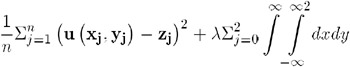
• For each value of the smoothing parameter, a function u ( x , y ) is formed that minimizes

• 

• where n is the number of data points and the pairs ( x _j , y _j )are the available points, with corresponding function values z _j (Wahba 1979).

  The higher the value of the smoothing parameter, the smoother the resulting interpolation. The lower the smoothing parameter, the closer the resulting surface is to the original data points. A smoothing parameter of 0 produces the same results as the SPLINE option without SMOOTH=.

  This procedure repeats for each value of the smoothing parameter. The output data set that you specify in the OUT= option contains the interpolated values, the values of the grid points, and the values of the smoothing parameter in the variable _SMTH_. The output data set contains a separate grid for each value of the smoothing parameter.

• Featured in: Example 2 on page 1339

SPLINE

• specifies the use of a bivariate spline (Harder and Desmarais 1972, Meinguet 1979) to interpolate or to form a smoothed estimate if you also use the SMOOTH= option. This option results in the use of an order n ³ algorithm, where n is the number of input data points. Consequently, this method can be time-consuming . If you use more than 100 input points, the procedure may use excessive time.

• Featured in: Example 2 on page 1339 and Example 4 on page 1343

Controlling Observations in the Output Data Set

By default, the G3GRID procedure produces a data set with 121 observations for combinations of 11 values for each of the horizontal variables, x and y . To create a data set with a different number of observations, use the GRID statement s NAXIS1= or NAXIS2= options to specify the number of the values of y or x , respectively. Or, use the GRID statement s AXIS1= or AXIS2= options to specify the actual values for y or x , respectively.

Table 47.1 on page 1336 shows the number of observations that will be in the output data set if you use any of these options.

Table 47.1: Number of Observations Contained in the Output Data Set

Options Specified	Number of Observations in Output Data Set
None	121
AXIS1=	(number of values for AXIS1=) * 11
AXIS2=	(number of values for AXIS2=) * 11
NAXIS1=	(value of NAXIS1=) * 11
NAXIS2=	(value of NAXIS2=) * 11
AXIS1=, AXIS2=	(number of values for AXIS1=) * (number of values for AXIS2=)
AXIS1=, NAXIS1=	(number of values for AXIS1=) * 11
AXIS1=, NAXIS2=	(number of values for AXIS1=) * (value of NAXIS2=)
AXIS2=, NAXIS1=	(number of values for AXIS2=) * (value of NAXIS1=)
AXIS2=, NAXIS2=	(number of values for AXIS2=) * 11
NAXIS1=, NAXIS2=	(value of NAXIS1=) * (value of NAXIS2=)

If you specify multiple smoothing parameters, the number of observations in the output data set will be the number shown in Table 47.1 on page 1336 multiplied by the number of smoothing values that you specify in the SMOOTH= option. If you use BY- group processing, multiply the number in the table by the number of BY groups.

Depending on the shape of the original data and the options that you specify, the output data set may contain values for the vertical ( z ) values that are outside of the range of the original values in the data set.