Section 11.4. Markovian FIFO Queueing Systems

11.4. Markovian FIFO Queueing Systems

In Markovian queueing systems, both arrival and service behaviors are based on Markovian-model queueing disciplines: M/M/ 1, M/M/ 1 /b , M/M/a , M/M/a/a , and M/M/ .

11.4.1. M/M/1 Queueing Systems

Figure 11.4 shows a simple queueing system model. Packets arrive according to a Poisson model at rate » so the interarrival times are IID exponential random variables with mean 1 /» . When the server is prepared for service, packets from the queue enter the server. Consider the situation in which the service times are IID exponential random variables with mean 1 / µ and the interarrival and service times are independent. With the M/M/ 1 model, it is in fact assumed that the system can accommodate an unlimited number of packets.

Figure 11.4. A simple queue/server model

Packet Arrival and Service Model

In an M/M/ 1 model, the packet arrival distribution is Poisson (see Appendix C) with rate » , or the interarrival time distribution is exponential with mean time 1 /» . Similarly, the service rate distribution is Poisson with rate µ , or the service time distribution is exponential with mean time 1 / µ . Note that the interarrival time and the service time are independent. Figure 11.5 shows an example in which five packets, A ₁ through A ₅ , arrive in random and require service times S ₁ through S ₅ , respectively. In this situation, queueing occurs while packets A ₃ and A ₄ wait in the buffer until the server becomes available. The probability that one packet arrives in an interval but no packet departs from the system is obtained using the Poisson formula:

Equation 11.12

Figure 11.5. Packet arrival, service, and departure

Equation (11.12) assumes that interval becomes very small and that therefore, all terms except the first one can be ignored. The same analysis can be derived for the case in which no packets arrive in an interval , but one packet departs from the system. Because one packet is serviced in an interval , we can use rate µ instead of » in Equation (11.12). Thus:

Equation 11.13

The last situation occurs when no change in the number of packets in the system is made. This means that there can be one arriving packet and one departing packet, or there can be no arriving packet and no departing packet. In either case, the probability can be derived by using Equations (11.12) and (11.13):

Equation 11.14

This analysis of the process is illustrated in Figure 11.6. In this process, a chain starts from a given state i , implying i packets in the system.

Figure 11.6. Packet arrival and departure

Number of Packets in the System

Properties obtained from Equations (11.12), (11.13), and (11.14) lead to the derivation of the number of packets in an M/M/ 1 system: K(t) . The fact is that K(t) follows a birth-and-death process, and its Markov chain follows exactly as the generic one shown in Figure 11.3 but with equal rates as modified in Figure 11.7. The main property of the exponential random variable implies that the interarrival time is independent of the present and past status of K(t) . Thus, if the system has K(t) > 0 packets, the interdeparture time distribution is also an exponential random variable. This also implies that the past history of the system is irrelevant for the probabilities of future states, and thus the process follows the property of a Markov chain. Note that M/M/ 1 is a simple case of a birth-death process with:

Equation 11.15

and

Equation 11.16

Figure 11.7. M/M/1 queueing behavior and its transitions

We define = ^» / _µ as the system utilization . The preceding Markov chain has the state-transition rate diagram shown in Figure 11.7, and its global balance equations for the steady-state probabilities can be set by using the birth-death process results simplified as

Equation 11.17

Since the sum of all probabilities is always 1, we can write

Equation 11.18

A stable situation exists when the arrival rate is less than the service rate, or = »/ µ < 1, in which case K(t) does not increase in value without bound, and therefore . This fact simplifies Equation (11.17) for the derivation of the number of packets in the system:

Equation 11.19

The condition = »/ µ < 1 must be met if the system is designed to be stable; otherwise , packets arrive at the system more quickly than they can be processed . It is apparent that if the packet-arrival rate exceeds the processing-capacity rate of servers, the number of packets in the queue grows without bound, leading to an unstable situation. Note that the distribution of K(t) follows a geometric distribution .

Mean Delay and Queue Length

The result derived from Equation (11.19) can be used to calculate the mean delay a packet spends in a queue or the entire system and the mean length of a queue. The average number of packets in the system is, in fact, the expected value of K(t) :

Equation 11.20

Little's formula can be used to derive the mean packet delay in the system:

Equation 11.21

We can now show the mean waiting time of a packet in the queue, E [ T _q ], in terms of E [ T ] and the mean processing time of a packet in the server, E [ T _s ]:

Equation 11.22

The mean processing time of a packet in the server, E [ T _s ], is in fact therefore:

Equation 11.23

Example.	Use Little's formula to find the mean number of packets in the queue.
Solution.	Little's formula can be applied in most stochastic systems, such as a queue defined solely as a system. If E [ K q (t) ] is the mean number of packets in the queue: Interestingly, the mean number of packets is a function only of utilization. In other words, the value of utilization in any single-queue system determines the average number of packets in the system.

11.4.2. Systems with Limited Queueing Space: M/M/1/b

In a queue with exponential interarrival times and exponential service times, a single server and a maximum of b packets can be held in the system. Once such a system exceeds its capacity, arriving packet numbered b + 1 is turned away from the system, since there is no room for it. Figure 11.8 shows the state-transition diagram for the M/M/ 1 /b system. This diagram is a Markov chain and is very similar to the one illustrated in Figure 11.7, but the chain for the M/M/ 1 /b system stops at the maximum capacity of b . Thus, the global balance equations use the same results presented in Equation(11.18), where the sum of all probabilities is always 1 and thus

Equation 11.24

Figure 11.8. State-transition diagram for M/M/ 1 /b system

A stable situation exists when the arrival rate is less than the service rate, or = »/ µ < 1, in which case K(t) does not increase in value without bound and therefore . This fact simplifies Equation (11.17) for deriving the number of packets in the system, which is a continuous-time Markov chain taking on values from the set {0, 1, ..., b }:

Equation 11.25

Note that the number of packets in the system is derived in two parts , depending on whether the utilization is maximized ( = 1) or not.

Mean Number of Packets

The mean number of packets in the system, E [ K(t) ], can be expressed by Formula C.20 in Appendix C:

Equation 11.26

Clearly, results of the mean number of packets in the M/M/ 1 and M/M/ 1 /b systems are fundamentally different, owing to the difference in capacities available in these two systems.

11.4.3. M/M/a Queueing Systems

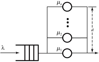
Some stochastic systems are modeled by M/M/a , where a servers instead of one can be used to enhance system performance, as shown in Figure 11.9. The service rate in each server may be different from or equal to that in the others, as rates µ ₁ through µ _a are indicated as service rates of the corresponding servers. The advantage of this discipline over systems with one server is its parallel-serving feature. A packet can be partitioned into i < a different tasks and served in parallel in i different servers concurrently.

Figure 11.9. Queueing model of M/M/a systems

The resulting system can be modeled by a continuous-time Markov chain, as shown in Figure 11.10. The maximum number of servers is denoted by a . As long as the number of packets in the queue is less than a , the service rate is proportionally changing ( i µ ) with the number of waiting packets while the arrival rate remains constant. However, when the number of packets in the queue reaches a , the arrival rate stays constant at its maximum of a µ .

Figure 11.10. State-transition diagram for M/M/a systems

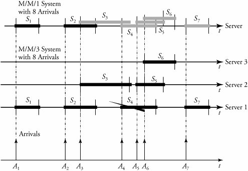
Example.

Figure 11.11 shows a statistical comparison between M/M/ 1 and M/M/ 3 systems, each with seven packets. In the M/M/ 1 system, the third packet, S ₃ , starts to accumulate in the queue. The queueing trend continues, as shown by gray, if the service rate stays low. On the contrary, in the M/M/ 3 system, packets are distributed over the three servers on arrival, and queueing has not happened .

Figure 11.11. Comparison of M/M/ 1 and M/M/ 3 systems, each with seven packets

Balance Equations for i a

The steady-state probabilities for the M/M/a system can be obtained by using the birth-and-death process. Balance equations for i servers being busy when i a begin with p _i :

Equation 11.27

Recall that is the utilization and that p _i = ( _{1 2} ... _{i - 1 i} )p . Thus, p _i can be rewritten as

Equation 11.28

It is easy to realize the probability that all servers are in use. Substitute i = a in Equation (11.28):

Equation 11.29

Balance Equations for i a

To determine the balance equations for i a , we again use the birth-and-death process. The second part of the transition diagram, starting from state a , is formulated over states i = a , a + 1, a + 2, .... As a result, the birth-and-death process formula is set up by

Equation 11.30

where = . In this equation, p _a can be substituted by the value obtained last from the case of i a , presented in Equation (11.29). Therefore, by replacing p _a with , we obtain

Equation 11.31

Equations (11.28) and (11.31) together cover all the cases in the state diagram. Since the sum of all probabilities is always 1,

Equation 11.32

To have a stable system, we want < 1, which causes to converge to . With this simplification, we can compute the probability of the first state from Equation 11.32:

Equation 11.33

Similar to previous cases, knowing p is essential, as we can derive p _i from Equation (11.31).

In an M/M/a system, we can use the Erlang-C formula to compute the blocking probability. This formula calculates the probability that an arriving packet finds all servers busy. This probability is the same as the probability that the waiting time for the packet in the queue is greater than zero, or the probability that the number of packets in the queueing system is greater than or equal to a , P [ K(t) a ]:

Equation 11.34

As with the M/M/ 1 queueing system, we can now estimate all the parameters for the M/M/a discipline. The mean number of packets in the queue is

Equation 11.35

Accordingly, the mean packet delay in the queue is

Equation 11.36

Obviously, the total mean packet delay in a system is

Equation 11.37

The mean number of packets in the system is obtained again from Little's formula:

Equation 11.38

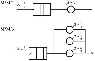
Example.	A communication node receives packets at » = 1/2 packet per nanosecond, and the switching server processes packets at the rate of one packet per nanosecond. Calculate the queueing delay and the total node's delay, and then compare the results for using queueing disciplines M/M/ 1 and M/M/ 3 with equal service powers as shown in Figure 11.12. Figure 11.12. Two queueing disciplines with equal service powers
Solution.	With an M/M/ 1 discipline, = »/ µ = 0.5. So the mean queueing delay is Equation 11.39 and the total node's delay is Equation 11.40 For the M/M/ 3 discipline, a = 3 servers are used; thus, 1 = »/ µ = 1.5, and = »/a µ = 0.5. Thus: Equation 11.41 Since , the queueing delay is Equation 11.42 and the total mean node's delay is Equation 11.43

This useful example expresses an important conclusion: Increasing the number of servers lowers the queueing delay but increases the total system delay. In summary, compared with the M/M/a system ( a> 1), the M/M/ 1 system has a smaller total delay but a larger queueing delay. However, note that the preceding statement should be made with an important condition; that is, the total service rates of a servers in the M/M/a model must be equal to the service rate of the M/M/ 1 model.

11.4.4. Models for Delay-Sensitive Traffic: M/M/a/a

Some network nodes can be built with no buffering elements. One application of such systems is for cases in which delay-sensitive traffic , such as voice, needs a queueless service. These types of nodes can be shown by queueless models. One example of such models is the M/M/a/a queueing system, which has a servers but no queueing line. If all servers are busy, an arriving packet is turned away, resulting in the transition-rate diagram shown in Figure 11.13. This transition rate partially resembles that for an M/M/a system. Thus, we use the previously obtained equation for the probability that the system is in state i ˆˆ{0, ..., a }:

Equation 11.44

Figure 11.13. State-transition diagram for M/M/a/a systems

Combining Equation (11.44) and the fact that gives us

Equation 11.45

Erlang-B Blocking Probability

In an M/M/a/a system, we can compute the blocking probability, this time using the Erlang-B formula . This formula calculates the probability that an arriving packet finds all servers busy but no waiting line for packets. The probability that all servers of the system are busy is referred to as the Erlang-B formula , using Equation (11.44) with i = a :

Equation 11.46

When all servers are busy, an incoming packet is turned away. Let » , » _p , and » _b = p _a » represent the arrival rate, the packet-passing rate, and the blocking rate, respectively. Therefore, » = » _p + » _b . The packet-passing rate can then be rewritten as » _p = »( 1 - p _a ) . In such systems, it would be interesting to find the average number of packets in the system, since no queueing line exists. From Little's formula:

Equation 11.47

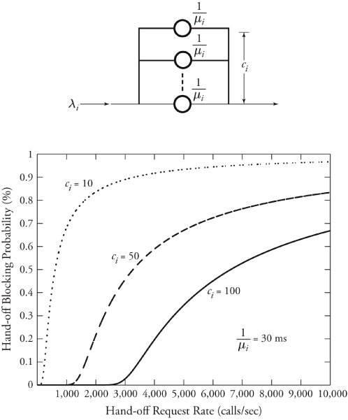
Example.

When a mobile user in a wireless data network moves to a new region, a handoff process between the two regions needs to take place. If all the new region's channels are used, the handoff call is terminated or blocked. For real-time communications, this scenario is modeled by an M/M/a/a system, where a = c i is the number of handoff servers of traffic type i . Assume that c i =10, 50, and 100; mean service time 1 / µ i = 30 msec; and handoff request rate » i = 0 ... 10, 000. Sketch a set of plots showing the performance of the handoff process.

Solution.

The calculation effort is left to readers. Instead, the results of the computations in Figure 11.14 are given. The plots in this figure depict the results of an M/M/a/a model for the wireless handoff. Equation (11.46) can be used to compute the handoff blocking probability. Figure 11.14. A wireless data network model as an M/M/a/a system with c i channel servers

11.4.5. M/M/ Queueing Systems

In many high-speed network nodes, higher cost can be tolerated in exchange for better communication quality. One method of improving the quality of handling packets is to consider a large number of servers at a node. If we let a approach a real large number approximated to infinity, an M/M/a/a system becomes an M/M/ system. As a result, the transition-rate diagram can continue to , as shown in Figure 11.15. To find steady-state probabilities, p _i , for this queueing system, we use Equation (11.46) of the M/M/a/a system and let a be a number i varying up to :

Equation 11.48

Figure 11.15. State-transition diagram for M/M/ system

In the denominator of this equation, tends to converge to e ¹ when i approaches infinity:

Equation 11.49