Details

Missing Values

A missing value for a parent implies that the parent is unknown. Unknown parents are assumed to be unrelated and not inbred unless you specify the INIT= option (see the INIT= option on page 1973).

When the value of the variable identifying the individual is missing, the observation is not added to the list of individuals. However, for a multiparous population, an observation with a missing individual is valid and is used for assigning covariances.

Missing covariance values are determined from the INIT= cov option, if specified. Observations with missing generation variables are excluded.

If the gender of an individual is missing, it is determined from the order in which it is listed on the first observation defining its progeny for an overlapping population. If it appears as the first parent, it is set to ˜M ; otherwise , it is set to ˜F . When the gender of an individual cannot be determined, it is assigned a default value of ˜F .

DATA= Data Set

Each observation in the input data set should contain necessary information such as the identification of an individual and the first and second parents of an individual. In addition, if a CLASS statement is specified, each observation should contain the generation identification; and, if a GENDER statement is specified, each observation should contain the gender of an individual. Optionally, each observation may also contain the covariance between the first and the second parents. Depending on how many statements are specified with the procedure, there should be enough variables in the input data set containing this information.

If you omit the VAR statement, then the procedure uses the first three unaddressed variables in the input data set as the names of the individual and his or her parents. Unaddressed variables in the input data set are those variables that are not referenced by the procedure in any other statements, such as CLASS, GENDER,orBY statements. If the input data set contains an unaddressed fourth variable, then the procedure uses it as the covariance variable.

If the individuals given by the variables associated with the first and second parents are not in the population, they are added to the population. However, if they are in the population, they must be defined prior to the observation that gives their progeny.

When there is a CLASS statement, the functions of defining new individuals and assigning covariances must be separated. This is necessary because the parents of any given individual are defined in the previous generation, while covariances are assigned between individuals in the current generation.

Therefore, there could be two types of observations for a multiparous population:

• one to define new individuals in the current generation whose parents have been defined in the previous generation, as in the following, where the missing value is for the covariance variable:

    MARK  GEORGE LISA . M 1   KELLY SCOTT  LISA . F 1  

• one to assign covariances between two individuals in the current generation, as in the following, where the individual s name is missing, ˜MARK and ˜KELLY are in the current generation, and the covariance coefficient between these two individuals is 0.50:

    . MARK KELLY 0.50 . 1  

Note that the observations defining individuals must precede the observation assigning a covariance value between them. For example, if a covariance is to be assigned between ˜MARK and ˜KELLY , then both of them should be defined prior to the assignment observation.

Computational Details

This section describes the rules that the INBREED procedure uses to compute the covariance and inbreeding coefficients. Each computational rule is explained by an example referring to the fictitious population introduced in the Getting Started section on page 1967.

Coancestry (or Kinship Coefficient)

To calculate the inbreeding coefficient and the covariance coefficients, use the degree of relationship by descent between the two parents, which is called coancestry or kinship coefficient (Falconer and Mackay 1996, p.85), or coefficient of parentage (Kempthorne 1957, p.73). Denote the coancestry between individuals X and Y by f _XY . For information on how to calculate the coancestries among a population, see the section Calculation of Coancestry.

Covariance Coefficient (or Coefficient of Relationship)

The covariance coefficient between individuals X and Y is defined by

where f _XY is the coancestry between X and Y. The covariance coefficient is sometimes called the coefficient of relationship or the theoretical correlation (Falconer and Mackay 1996, p.153; Crow and Kimura 1970, p.134). If a covariance coefficient cannot be calculated from the individuals in the population, it is assigned to an initial value. The initial value is set to 0 if the INIT= option is not specified or to cov if INIT= cov . Therefore, the corresponding initial coancestry is set to 0 if the INIT= option is not specified or to 1/2 cos if INIT= cov .

Inbreeding Coefficients

The inbreeding coefficient of an individual is the probability that the pair of alleles carried by the gametes that produced it are identical by descent (Falconer and Mackay 1996, Chapter 5; Kempthorne 1957, Chapter 5). For individual X, denote its inbreeding coefficient by F _X . The inbreeding coefficient of an individual is equal to the coancestry between its parents. For example, if X has parents A and B, then the inbreeding coefficient of X is

Calculation of Coancestry

Given individuals X and Y, assume that X has parents A and B and that Y has parents C and D. For nonoverlapping generations, the basic rule to calculate the coancestry between X and Y is given by the following formula (Falconer and Mackay 1996, p.86):

And the inbreeding coefficient for an offspring of X and Y, called Z, is the coancestry between X and Y:

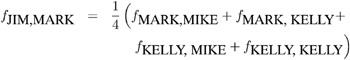
For example, in Figure 35.4, ˜JIM and ˜MARK from Generation 2 are progenies of ˜MARK and ˜KELLY and of ˜MIKE and ˜KELLY from Generation 1, respectively. The coancestry between ˜JIM and ˜MARK is

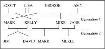
Figure 35.4: Inbreeding Relationship for Nonoverlapping Population

From the covariance matrix for Generation =1 in Figure 35.2 (page 1971) and the relationship that coancestry is half of the covariance coefficient,

For overlapping generations, if X is older than Y, then the basic rule (on page 1978) can be simplified to

That is, the coancestry between X and Y is the average of coancestries between older X with younger Y s parents. For example, in Figure 35.5, the coancestry between ˜KELLY and ˜DAVID is

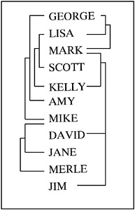
Figure 35.5: Inbreeding Relationship for Overlapping Population

This is so because ˜KELLY is defined before ˜DAVID ; therefore, ˜KELLY is not younger than ˜DAVID , and the parents of ˜DAVID are ˜MARK and ˜KELLY . The covariance coefficient values Cov(KELLY,MARK) and Cov(KELLY,KELLY) from the matrix in Figure 35.1 on page 1970 yield that the coancestry between ˜KELLY and ˜DAVID is

The numerical values for some initial coancestries must be known in order to use these rule. Either the parents of the first generation have to be unrelated, with f = 0 if the INIT= option is not specified in the PROC statement, or their coancestries must have an initial value of 1/2 cos , where cov is set by the INIT= option. Then the subsequent coancestries among their progenies and the inbreeding coefficients of their progenies in the rest of the generations are calculated using these initial values.

Special rules need to be considered in the calculations of coancestries for the following cases.

Self-Mating

The coancestry for an individual X with itself, f _XX , is the inbreeding coefficient of a progeny that is produced by self-mating. The relationship between the inbreeding coefficient and the coancestry for self-mating is

The inbreeding coefficient F _X can be replaced by the coancestry between X s parents A and B, f _AB , if A and B are in the population:

If X s parents are not in the population, then F _X is replaced by the initial value 1/2 cov if cov is set by the INIT= option, or F _X is replaced by 0 if the INIT= option is not specified. For example, the coancestry of ˜JIM with himself is

where ˜MARK and ˜KELLY are the parents of ˜JIM . Since the covariance coefficient Cov(MARK,KELLY) is 0.5 in Figure 35.1 on page 1970 and also in the covariance matrix for GENDER=1 in Figure 35.2 on page 1971, the coancestry of ˜JIM with himself is

When INIT=0.25, then the coancestry of ˜JANE with herself is

because ˜JANE is not an offspring in the population.

Offspring and Parent Mating

Assuming that X s parents are A and B, the coancestry between X and A is

The inbreeding coefficient for an offspring of X and A, denoted by Z, is

For example, ˜MARK is an offspring of ˜GEORGE and ˜LISA , so the coancestry between ˜MARK and ˜LISA is

From the covariance coefficient matrix in Figure 35.1 on page 1970, f _LISA,GEORGE = 0 . 25 / 2 = 0 . 125, f _LISA,LISA = 1 . 125 / 2 = 0 . 5625 , so that

Thus, the inbreeding coefficient for an offspring of ˜MARK and ˜LISA is 0.34375.

Full Sibs Mating

This is a special case for the basic rule given at the beginning of the section Calculation of Coancestry on page 1978. If X and Y are full sibs with same parents A and B, then the coancestry between X and Y is

and the inbreeding coefficient for an offspring of A and B, denoted by Z, is

For example, ˜DAVID and ˜JIM are full sibs with parents ˜MARK and ˜KELLY , so the coancestry between ˜DAVID and ˜JIM is

Since the coancestry is half of the covariance coefficient, from the covariance matrix in Figure 35.1 on page 1970,

Unknown or Missing Parents

When individuals or their parents are unknown in the population, their coancestries are assigned by the value 1/2 cov if cov is set by the INIT= option or by the value 0 if the INIT= option is not specified. That is, if either A or B is unknown, then

For example, ˜JANE is not in the population, and since ˜JANE is assumed to be defined just before the observation at which ˜JANE appears as a parent (that is, between observations 4 and 5), then ˜JANE is not older than ˜SCOTT . The coancestry between ˜JANE and ˜SCOTT is then obtained by using the simplified basic rule (see page 1979):

Here, dots ( ·) indicate JANE s unknown parents. Therefore, f _SCOTT, . is replaced by 1/2 cov , where cov is set by the INIT= option. If INIT=0.25, then

For a more detailed discussion on the calculation of coancestries, inbreeding coefficients, and covariance coefficients, refer to Falconer and Mackay (1996), Kempthorne (1957), and Crow and Kimura (1970).

OUTCOV= Data Set

The OUTCOV= data set has the following variables:

• a list of BY variables, if there is a BY statement

• the generation variable, if there is a CLASS statement

• the gender variable, if there is a GENDER statement

• _ Type_ , a variable indicating the type of observation. The valid values of the _ Type_ variable are ˜COV for covariance estimates and ˜INBREED for inbreeding coefficients.

• _ Panel_ , a variable indicating the panel number used when populations delimited by BY groups contain different numbers of individuals. If there are n individuals in the first BY group and if any subsequent BY group contains a larger population, then its covariance/inbreeding matrix is divided into panels, with each panel containing n columns of data. If you put these panels side by side in increasing _ Panel_ number order, then you can reconstruct the covariance or inbreeding matrix.

• _ Col_ , a variable used to name columns of the inbreeding or covariance matrix. The values of this variable start with ˜COL , followed by a number indicating the column number. The names of the individuals corresponding to any given column i can be found by reading the individual s name across the row that has a _ Col_ value of ˜COL i . When the inbreeding or covariance matrix is divided into panels, all the rows repeat for the first n columns, all the rows repeat for the next n columns, and so on.

• the variable containing the names of the individuals, that is, the first variable listed in the VAR statement

• the variable containing the names of the first parents, that is, the second variable listed in the VAR statement

• the variable containing the names of the second parents, that is, the third variable listed in the VAR statement

• a list of covariance variables Col1 - Col n , where n is the maximum number of individuals in the first population

The functions of the variables _ Panel_ and _ Col_ can best be demonstrated by an example. Assume that there are three individuals in the first BY group and that, in the current BY group ( Byvar =2), there are five individuals with the following covariance matrix.

COV	1	2	3	4	5
1	Cov(1,1)	Cov(1,2)	Cov(1,3)	Cov(1,4)	Cov(1,5)
2	Cov(2,1)	Cov(2,2)	Cov(2,3)	Cov(2,4)	Cov(2,5)
3	Cov(3,1)	Cov(3,2)	Cov(3,3)	Cov(3,4)	Cov(3,5)
4	Cov(4,1)	Cov(4,2)	Cov(4,3)	Cov(4,4)	Cov(4,5)
5	Cov(5,1)	Cov(5,2)	Cov(5,3)	Cov(5,4)	Cov(5,5)
	Panel 1			Panel 2

Then the OUTCOV= data set appears as follows .

Byvar	_ Panel_	_ Col_	Individual	Parent	Parent2	Col1	Col2	Col3
2	1	COL1	1			Cov(1,1)	Cov(1,2)	Cov(1,3)
2	1	COL2	2			Cov(2,1)	Cov(2,2)	Cov(2,3)
2	1	COL3	3			Cov(3,1)	Cov(3,2)	Cov(3,3)
2	1		4			Cov(4,1)	Cov(4,2)	Cov(4,3)
2	1		5			Cov(5,1)	Cov(5,2)	Cov(5,3)
2	2		1			Cov(1,4)	Cov(1,5)	.
2	2		2			Cov(2,4)	Cov(2,5)	.
2	2		3			Cov(3,4)	Cov(3,5)	.
2	2	COL1	4			Cov(4,4)	Cov(4,5)	.
2	2	COL2	5			Cov(5,4)	Cov(5,5)	.

Notice that the first three columns go to the first panel ( _ Panel_ =1), and the remaining two go to the second panel ( _ Panel_ =2). Therefore, in the first panel, ˜COL1 , ˜COL2 , and ˜COL3 correspond to individuals 1, 2, and 3, respectively, while in the second panel, ˜COL1 and ˜COL2 correspond to individuals 4 and 5, respectively.

Displayed Output

The INBREED procedure can output either covariance coefficients or inbreeding coefficients. Note that the following items can be produced for each generation if generations do not overlap.

The output produced by PROC INBREED can be any or all of the following items:

• a matrix of coefficients

• coefficients of the individuals

• coefficients for selected matings

ODS Table Names

PROC INBREED assigns a name to each table it creates. You can use these names to reference the table when using the Output Delivery System (ODS) to select tables and create output data sets. These names are listed in the following table.

For more information on ODS, see Chapter 14, Using the Output Delivery System.

Table 35.1: ODS Tables Produced in PROC INBREED

ODS Table Name	Description	Statement	Option
AvgCovCoef	Averages of covariance coefficient matrix	GENDER	COVAR and AVERAGE
AvgInbreedingCoef	Averages of inbreeding coefficient matrix	GENDER	AVERAGE
CovarianceCoefficient	Covariance coefficient table	PROC	COVAR and MATRIX
InbreedingCoefficient	Inbreeding coefficient table	PROC	MATRIX
IndividualCovCoef	Covariance coefficients of individuals	PROC	IND and COVAR
IndividualInbreedingCoef	Inbreeding coefficients of individuals	PROC	IND
MatingCovCoef	Covariance coefficients of matings	MATINGS	COVAR
MatingInbreedingCoef	Inbreeding coefficients of matings	MATINGS
NumberOfObservations	Number of observations	PROC