Section 31. Normality Test

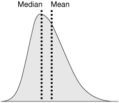
31. Normality Test

Overview

The Normality Test is used on a sample of data to determine the likelihood of the population from which the sample originates being normally distributed. The result would be a degree of confidence in the population being normally distributed (a p-value).

Normality is crucial for the majority of statistical tests examining the means and variances of samples. For example, if data becomes skewed (thus, non-normal), then the mean is probably not the best measure of center and a median-based test is probably better. The longer tail on the right of the example curve in Figure 7.31.1 drags the mean to the right; however, the median tends to remain constant.

Figure 7.31.1. The effect of Normality on measures of center.

Roadmap

The hypotheses for a Normality Test are

• H₀: Population (process) data are normal

• H_a: Population (process) data are non-normal

The test is applied to a column of data (the sample) and the results obtained.

Interpreting the Output

There are a number of Normality Tests, for example those listed in Minitab include (with simple descriptions in English):

• Anderson-Darling Examines the area between the sample data distribution and the normal distribution (smaller the better).

• Ryan-Joiner^[53] Examines the correlation between the sample data and a normal distribution (the more correlated the better). This is useful for small sample sizes.

• Kolmogorov-Smirnov Similarly to the Anderson-Darling Test, examines the area between the sample data distribution and the normal distribution (smaller the better).

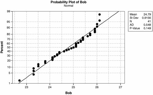
To be candid, in the world of Process Improvement there really won't be a dramatic difference in conclusion based on the tests. It is advisable to stick with one and the default in Minitab is Anderson-Darling, so I personally tend to run with that one.

Each test returns a test statistic, but the thing to be most interested in is the p-value, the likelihood that for the sample data a level of non-normality this large could have occurred purely by random chance even if the population were normally distributed.

Output from a Normality Test is shown in Figure 7.31.2.

Figure 7.31.2. Normality Test (Anderson-Darling) results for a sample of Bob's time to perform a task (output from Minitab v14).

The vertical scale on the graph is non-linear and the horizontal axis is a linear scale, similar to normal probability paper. If the data were perfectly normally distributed then the points would lay exactly on the line (and the p-value, in this case, theoretically should be 1.0).

From the example results:

• The sample mean is 24.79 (and this represents the best available approximation to the population mean).

• The sample standard deviation is 0.9156 (and this represents the best available approximation to the population standard deviation).

• The sample was made up of 41 data points.

• The Anderson-Darling statistic is 0.548 (remember the lower the better) with the likelihood of seeing a statistic this large, if the parent population were normally distributed, being 14.9% (p-value).

The hypotheses for a Normality Test are

• H₀: Population (process) data are normal

• H_a: Population (process) data are non-normal

The p-value should be interpreted in the usual way:

• p less than 0.05reject H₀ and conclude that the data are non-normal

• p greater than 0.05accept H₀ and conclude that the data are normal

Therefore, for Bob's data, shown in Figure 7.31.2 with a p-value of 0.149, which is clearly greater than 0.05, the conclusion should be that Bob's data are normal.