Constrained Optimization

[Page 455 ( continued )]

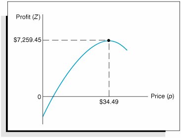
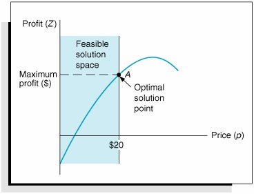
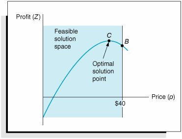
In the preceding section, the profit analysis model was developed as an extension of the break-even model. Recall that the total profit function was

Z = vp c _f vc _v

where

v = volume

p = price

c _f = fixed cost

c _v = variable cost

and the demand function (i.e., volume as a function of price) was

v = 1,500 24.6 p

By substituting this demand function into our total profit equation, we developed a non-linear function:

Z = 1,500 p 24.6 p ² c _f 1,500 c _v + 24.6 pc _v

Then, by substituting values for c _f ($10,000) and c _v ($8) into this function, we obtained

Z = 1,696.8 p 24.6 p ² 22,000

We then differentiated this function, set it equal to zero, and solved for the value of p ($34.49), which corresponded to the maximum point on the profit curve (where the slope equaled zero).

This type of model is referred to as an unconstrained optimization model . It consists of a single nonlinear objective function and no constraints. If we add one or more constraints to this model, it becomes a constrained optimization model . A constrained optimization model is more commonly referred to as a nonlinear programming model . The reason this type of model is designated as a form of mathematical programming is because all types of mathematical programming models are actually constrained optimization models. That is, they all have the general form of an objective function that is subject to one or more constraints . Linear programming has an objective function and constraints that happen to be linear. A nonlinear programming model has the same general form as a linear programming model, except that the objective function and/or the constraint(s) are nonlinear.

---

[Page 456]

Nonlinear programming differs from linear programming, however, in one other critical aspect: The solution of nonlinear programming problems is much more complex. In linear programming a particular procedure is guaranteed to lead to a solution if the problem has been correctly formulated, whereas in nonlinear programming no guaranteed procedure exists. The reason for this complexity can be illustrated by a graph of our profit analysis model. Figure 10.5 shows the nonlinear profit curve for the example model.

Figure 10.5. Nonlinear profit curve for the profit analysis model

As stated previously, the solution is found by taking the derivative of the profit function, setting it equal to zero, and solving for p (price). This results in an optimal value for p that corresponds to the maximum profit, as shown in Figure 10.5.

Now we will transform this unconstrained optimization model into a nonlinear programming model by adding the constraint

p $20

In other words, because of market conditions, we are restricting the price to a maximum of $20. This constraint results in a feasible solution space, as shown in Figure 10.6.

As in a linear programming problem, the solution is on the boundary of the feasible solution space formed by the constraint. Thus, in Figure 10.6, point A is the optimal solution. It corresponds to the maximum value of the portion of the objective function that is still feasible. However, the difficulty with nonlinear programming is that the solution is not always on the boundary of the feasible solution space formed by the constraint. For example, consider the addition of the following constraint to our original nonlinear objective function:

p $40

---

[Page 457]

Figure 10.6. A constrained optimization model

This constraint also creates a feasible solution space, as shown in Figure 10.7.

Figure 10.7. A constrained optimization model with a solution point not on the constraint boundary

But notice in Figure 10.7 that the solution is no longer on the boundary of the feasible solution space, as it would be in linear programming. Point C represents a greater profit than point B , and it is also in the feasible solution space. This means that we cannot simply look at points on the solution space boundary to find the solution; instead, we must also consider other points on the surface of the objective function. This greatly complicates the process of finding a solution to a nonlinear programming problem, and this difficulty is aggravated by an increased number of variables and constraints and by nonlinear functions of a higher order. You can imagine the difficulties of solution if you contemplate a model in space that is made up of intersecting cones, ellipses, and undulating surfaces, as well as planes, and a solution that is not even on the boundary of the solution space.

A number of different solution approaches to nonlinear programming problems are available. As we have already indicated, they typically represent a convergence of the principles of calculus and mathematical programming. However, as noted earlier, the solution techniques can be very complex. Thus, we will confine our discussion of nonlinear programming solution methods to several different model applications and the Excel solution.

---

[Page 458]