Examples
Example 30.1. Generalized Additive Model with Binary Data
The following example illustrates the capabilities of the GAM procedure and compares it to the GENMOD procedure.
The data used in this example are based on a study by Bell et al. (1994). Bell and his associates studied the result of multiple-level thoracic and lumbar laminectomy, a corrective spinal surgery commonly performed on children. The data in the study consist of retrospective measurements on 83 patients . The specific outcome of interest is the presence (1) or absence (0) of kyphosis, defined as a forward flexion of the spine of at least 40 degrees from vertical. The available predictor variables are Age in months at time of the operation, the starting of vertebrae levels involved in the operation ( StartVert ), and the number of levels involved ( NumVert ). The goal of this analysis is to identify risk factors for kyphosis. PROC GENMOD can be used to investigate the relationship among kyphosis and the predictors. The following DATA step creates the data kyphosis :
title 'Comparing PROC GAM with PROC GENMOD'; data kyphosis; input Age StartVert NumVert Kyphosis @@; datalines; 71 5 3 0 158 14 3 0 128 5 4 1 2 1 5 0 1 15 4 0 1 16 2 0 61 17 2 0 37 16 3 0 113 16 2 0 59 12 6 1 82 14 5 1 148 16 3 0 18 2 5 0 1 12 4 0 243 8 8 0 168 18 3 0 1 16 3 0 78 15 6 0 175 13 5 0 80 16 5 0 27 9 4 0 22 16 2 0 105 5 6 1 96 12 3 1 131 3 2 0 15 2 7 1 9 13 5 0 12 2 14 1 8 6 3 0 100 14 3 0 4 16 3 0 151 16 2 0 31 16 3 0 125 11 2 0 130 13 5 0 112 16 3 0 140 11 5 0 93 16 3 0 1 9 3 0 52 6 5 1 20 9 6 0 91 12 5 1 73 1 5 1 35 13 3 0 143 3 9 0 61 1 4 0 97 16 3 0 139 10 3 1 136 15 4 0 131 13 5 0 121 3 3 1 177 14 2 0 68 10 5 0 9 17 2 0 139 6 10 1 2 17 2 0 140 15 4 0 72 15 5 0 2 13 3 0 120 8 5 1 51 9 7 0 102 13 3 0 130 1 4 1 114 8 7 1 81 1 4 0 118 16 3 0 118 16 4 0 17 10 4 0 195 17 2 0 159 13 4 0 18 11 4 0 15 16 5 0 158 15 4 0 127 12 4 0 87 16 4 0 206 10 4 0 11 15 3 0 178 15 4 0 157 13 3 1 26 13 7 0 120 13 2 0 42 6 7 1 36 13 4 0 ; proc genmod; model Kyphosis = Age StartVert NumVert / link=logit dist=binomial; run;
The GENMOD analysis of the independent variable effects is shown in Output 30.1.1. Based on these results, the only significant factor is StartVert with a log odds ratio of ˆ’ . 1972. The variable NumVert has a p -value of 0.0904 with a log odds ratio of 0 . 3031.
| |
Comparing PROC GAM with PROC GENMOD The GENMOD Procedure PROC GENMOD is modeling the probability that Kyphosis='0'. One way to change this to model the probability that Kyphosis='1' is to specify the DESCENDING option in the PROC statement. Analysis Of Parameter Estimates Standard Wald 95% Chi- Parameter DF Estimate Error Confidence Limits Square Pr > ChiSq Intercept 1 1.2497 1.2424 1.1853 3.6848 1.01 0.3145 Age 1 0.0061 0.0055 0.0170 0.0048 1.21 0.2713 StartVert 1 0.1972 0.0657 0.0684 0.3260 9.01 0.0027 NumVert 1 0.3031 0.1790 0.6540 0.0477 2.87 0.0904 Scale 0 1.0000 0.0000 1.0000 1.0000 NOTE: The scale parameter was held fixed.
| |
The GENMOD procedure assumes a strict linear relationship between the response and the predictors. The following SAS statements use PROC GAM to investigate a less restrictive model, with moderately flexible spline terms for each of the predictors:
title 'Comparing PROC GAM with PROC GENMOD'; proc gam data=kyphosis; model Kyphosis = spline(Age ,df=3) spline(StartVert,df=3) spline(NumVert ,df=3) / dist=binomial; run;
The MODEL statement requests an additive model using a univariate smoothing spline for each term . The option dist=binomial with binary responses specifies a logistic model. Each term is fit using a univariate smoothing spline with three degrees of freedom. Of these three degrees of freedom, one is taken up by the linear portion of the fit and two are left for the nonlinear spline portion. Although this might seem to be an unduly modest amount of flexibility, it is better to be conservative with a data set this small.
Output 30.1.2 and Output 30.1.3 list the output from PROC GAM.
| |
Comparing PROC GAM with PROC GENMOD The GAM Procedure Dependent Variable: Kyphosis Smoothing Model Component(s): spline(Age) spline(StartVert) spline(NumVert) Summary of Input Data Set Number of Observations 83 Number of Missing Observations 0 Distribution Binomial Link Function Logit Iteration Summary and Fit Statistics Number of local score iterations 9 Local score convergence criterion 2.6635657E-9 Final Number of Backfitting Iterations 1 Final Backfitting Criterion 5.2326588E-9 The Deviance of the Final Estimate 46.610922438
| |
| |
Comparing PROC GAM with PROC GENMOD The GAM Procedure Dependent Variable: Kyphosis Smoothing Model Component(s): spline(Age) spline(StartVert) spline(NumVert) Regression Model Analysis Parameter Estimates Parameter Standard Parameter Estimate Error t Value Pr > t Intercept 2.01533 1.45620 1.38 0.1706 Linear(Age) 0.01213 0.00794 1.53 0.1308 Linear(StartVert) 0.18615 0.07628 2.44 0.0171 Linear(NumVert) 0.38347 0.19102 2.01 0.0484 Smoothing Model Analysis Fit Summary for Smoothing Components Num Smoothing Unique Component Parameter DF GCV Obs Spline(Age) 0.999996 2.000000 328.512831 66 Spline(StartVert) 0.999551 2.000000 317.646685 16 Spline(NumVert) 0.921758 2.000000 20.144056 10 Smoothing Model Analysis Analysis of Deviance Sum of Source DF Squares Chi Square Pr > ChiSq Spline(Age) 2.00000 10.494369 10.4944 0.0053 Spline(StartVert) 2.00000 5.494968 5.4950 0.0641 Spline(NumVert) 2.00000 2.184518 2.1845 0.3355
| |
ods html; ods graphics on; proc gam data=kyphosis plots(clm commonaxes); model Kyphosis = spline(Age ,df=3) spline(StartVert,df=3) spline(NumVert ,df=3) / dist=binomial; run; ods graphics off; ods html close;
For general information about ODS graphics, see Chapter 15, Statistical Graphics Using ODS. For specific information about the graphics available in the GAM procedure, see the section ODS Graphics on page 1581. The smoothing component plots are displayed in Output 30.1.4.
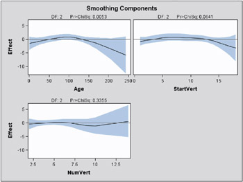
The plots show that the partial predictions corresponding to both Age and StartVert have a quadratic pattern, while NumVert has a more complicated but weaker pattern. However, in the plot for NumVert , notice that about half the vertical range of the function is determined by the point at the upper extreme. It would be a good idea, therefore, to rerun the analysis without this point, to explore how much it affects the conclusions. You can do this by simply including a WHERE clause when specifying the data set for the GAM procedure, as in the following code:
ods html; ods graphics on; proc gam data=kyphosis(where=(NumVert^=14)) plots(clm commonaxes); model Kyphosis = spline(Age ,df=3) spline(StartVert,df=3) spline(NumVert ,df=3) / dist=binomial; run; ods graphics off; ods html close;
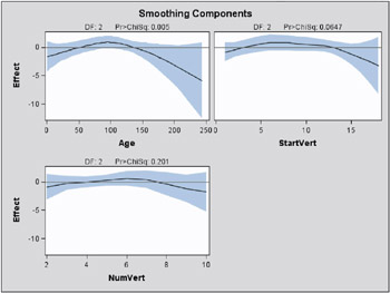
The analysis of deviance table from this reanalysis is shown in Output 30.1.5, and Output 30.1.6 shows the recomputed partial predictor plots.
| |
Comparing PROC GAM with PROC GENMOD The GAM Procedure Dependent Variable: Kyphosis Smoothing Model Component(s): spline(Age) spline(StartVert) spline(NumVert) Smoothing Model Analysis Analysis of Deviance Sum of Source DF Squares Chi-Square Pr > ChiSq Spline(Age) 2.00000 10.587556 10.5876 0.0050 Spline(StartVert) 2.00000 5.477094 5.4771 0.0647 Spline(NumVert) 2.00000 3.209089 3.2091 0.2010
| |
| |
| |
Removing data point NumVert =14 has little effect on either the analysis of deviance results or the estimated curves for StartVert and NumVert . But the removal has a noticeable effect on the variable NumVert , whose curve now also seems quadratic, though it is much less pronounced than for the other two variables.
An important difference between the first analysis of this data with GENMOD and the subsequent analysis with GAM is that GAM indicates that age is a significant predictor of kyphosis. The difference is due to the fact that the GENMOD model only includes a linear effect in Age whereas the GAM model allows a more complex relationship, which the plots indicate is nearly quadratic. Having used the GAM procedure to discover an appropriate form of the dependence of Kyphosis on each of the three independent variables, you can use the GENMOD procedure to fit and assess the corresponding parametric model. The following code fits a GENMOD model with quadratic terms for all three variables, including tests for the joint linear and quadratic effects of each variable. The resulting contrast tests are shown in Output 30.1.7.
| |
Comparing PROC GAM with PROC GENMOD The GENMOD Procedure PROC GENMOD is modeling the probability that Kyphosis='0'. One way to change this to model the probability that Kyphosis='1' is to specify the DESCENDING option in the PROC statement. Contrast Results Chi- Contrast DF Square Pr > ChiSq Type Age 2 13.63 0.0011 LR StartVert 2 15.41 0.0005 LR NumVert 2 3.56 0.1684 LR
| |
title 'Comparing PROC GAM with PROC GENMOD'; proc genmod data=kyphosis(where=(NumVert^=14)); model kyphosis = Age Age *Age StartVert StartVert*StartVert NumVert NumVert *NumVert /link=logit dist=binomial; contrast 'Age' Age 1, Age*Age 1; contrast 'StartVert' StartVert 1, StartVert*StartVert 1; contrast 'NumVert' NumVert 1, NumVert*NumVert 1; run;
The results for the quadratic GENMOD model are now quite consistent with the GAM results.
From this example, you can see that PROC GAM is very useful in visualizing the data and detecting the nonlinearity among the variables.
Example 30.2. Poisson Regression Analysis of Component Reliability
In this example, the number of maintenance repairs on a complex system are modeled as realizations of Poisson random variables. The system under investigation has a large number of components, which occasionally break down and are replaced or repaired. During a four-year period, the system was observed to be in a state of steady operation, meaning that the rate of operation remained approximately constant. A monthly maintenance record is available for that period, which tracks the number of components removed for maintenance each month. The data are listed in the following statements that create a SAS data set.
title 'Analysis of Component Reliability'; data equip; input year month removals @@; datalines; 1987 1 2 1987 2 4 1987 3 3 1987 4 3 1987 5 3 1987 6 8 1987 7 2 1987 8 6 1987 9 3 1987 10 9 1987 11 4 1987 12 10 1988 1 4 1988 2 6 1988 3 4 1988 4 4 1988 5 3 1988 6 5 1988 7 3 1988 8 4 1988 9 5 1988 10 3 1988 11 6 1988 12 3 1989 1 2 1989 2 6 1989 3 1 1989 4 5 1989 5 5 1989 6 4 1989 7 2 1989 8 2 1989 9 2 1989 10 5 1989 11 1 1989 12 10 1990 1 3 1990 2 8 1990 3 12 1990 4 7 1990 5 3 1990 6 2 1990 7 4 1990 8 3 1990 9 0 1990 10 6 1990 11 6 1990 12 6 ; run;
For planning purposes, it is of interest to understand the long- and short-term trends in the maintenance needs of the system. Over the long term, it is suspected that the quality of new components and repair work improves over time, so the number of component removals would tend to decrease from year to year. It is not known whether the robustness of the system is affected by seasonal variations in the operating environment, but this possibility is also of interest.
Because the maintenance record is in the form of counts, the number of removals are modeled as realizations of Poisson random variables. Denote by » ij the unobserved component removal rate for year i and month j . Since the data were recorded at regular intervals (from a system operating at a constant rate), each » ij is assumed to be a function of year and month only.
A preliminary two-way analysis is performed using PROC GENMOD to make broad inferences on repair trends. A log-link is specified for the model
where µ is a grand mean, ![]() is the effect of the i th year, and
is the effect of the i th year, and ![]() is the effect of the j th month. A CLASS statement declares the variables year and month as categorical. Type III sum of squares are requested to test whether there is an overall effect of year and/or month.
is the effect of the j th month. A CLASS statement declares the variables year and month as categorical. Type III sum of squares are requested to test whether there is an overall effect of year and/or month.
title2 'Two-way model'; proc genmod data=equip; class year month; model removals=year month / dist=Poisson link=log type3; run;
| |
Analysis of Component Reliability Two-way model The GENMOD Procedure LR Statistics For Type 3 Analysis Chi- Source DF Square Pr > ChiSq year 3 2.63 0.4527 month 11 21.12 0.0321
| |
The Type III tests indicate that the year term may be dropped from the model. The focus of the analysis is now on identifying the form of the underlying seasonal trend, which is a task that PROC GAM is especially suited for. PROC GAM will be used to fit both a reduced categorical model, with year eliminated, and a nonparametric spline model. Although PROC GENMOD also has the capability to fit categorical models, as demonstrated above, PROC GAM will be used to fit both models for a better comparison.
The following PROC GAM statements specify the reduced categorical model. For this part of the analysis, a CLASS statement is again used to specify that month is a categorical variable. In the follow-up, the seasonal effect will be treated as a nonparametric function of month .
title2 'One-way model'; proc gam data=equip; class month; model removals=param(month) / dist=Poisson; output out=est predicted; run;
The following statements generate a plot of the estimated seasonal trend. Note that the predicted values in the output data set correspond to the logarithms of the » ij , and so the exponential function is applied to put them on the scale of the original data. The plot is displayed in Output 30.2.2.
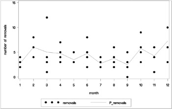
proc sort data=est out=plot; by month; run; data plot; set plot; P_removals = exp(P_removals); run; legend1 frame cframe=ligr cborder=black label=none position=center; axis1 minor=none order=(0 to 15 by 5) label=(angle=90 rotate=0 "number of removals"); axis2 minor=none label=("month"); symbol1 color=black interpol=none value=dot; symbol2 color=blue interpol=join value=none line=1; title; proc gplot data=plot; plot removals*month=1 P_removals*month=2 / overlay cframe=ligr legend=legend1 frame vaxis=axis1 haxis=axis2; run; quit; One advantage of nonparametric regression is its ability to highlight general trends in the data, such as those described above, and attribute local fluctuations to unexplained random noise. The nonparametric regression model used by PROC GAM specifies that the underlying removal rates » j are of the form
where ² 1 is a linear coefficient and s () is a nonparametric regression function. ² 1 and s () define the linear and nonparametric parts , respectively, of the seasonal trend.
The following statements request that PROC GAM fit a cubic spline model to the monthly repair data. The output listing is displayed in Output 30.2.3.
| |
Analysis of Component Reliability Spline model The GAM Procedure Dependent Variable: removals Smoothing Model Component(s): spline(month) Summary of Input Data Set Number of Observations 48 Number of Missing Observations 0 Distribution Poisson Link Function Log Iteration Summary and Fit Statistics Number of local score iterations 5 Local score convergence criterion 7.241527E-12 Final Number of Backfitting Iterations 1 Final Backfitting Criterion 1.710339E-11 The Deviance of the Final Estimate 56.901543546
| |
title 'Analysis of Component Reliability'; title2 'Spline model'; proc gam data=equip; model removals=spline(month) / dist=Poisson method=gcv; run;
The METHOD=GCV option is used to determine an appropriate level of smoothing. The keywords LCLM and UCLM in the OUTPUT statement request that lower and upper 95% confidence bounds on each s ( Month j ) be included in the output data set.
| |
Spline model The GAM Procedure Dependent Variable: removals Smoothing Model Component(s): spline(month) Regression Model Analysis Parameter Estimates Parameter Standard Parameter Estimate Error t Value Pr > t Intercept 1.34594 0.14509 9.28 <.0001 Linear(month) 0.02274 0.01893 1.20 0.2362 Smoothing Model Analysis Fit Summary for Smoothing Components Num Smoothing Unique Component Parameter DF GCV Obs Spline(month) 0.901512 1.879980 0.115848 12 Smoothing Model Analysis Analysis of Deviance Sum of Source DF Squares Chi-Square Pr > ChiSq Spline(month) 1.87998 8.877764 8.8778 0.0103
| |
The following statements use the experimental ODS GRAPHICS statement to plot the smoothing component for the effect of Month on predicted repair rates.
ods html; ods graphics on; proc gam data=equip; model removals=spline(month) / dist=Poisson method=gcv; run; ods graphics off; ods html close;
For general information about ODS graphics, see Chapter 15, Statistical Graphics Using ODS. For specific information about the graphics available in the GAM procedure, see the section ODS Graphics on page 1581. The smoothing component plot is displayed in Output 30.2.5.
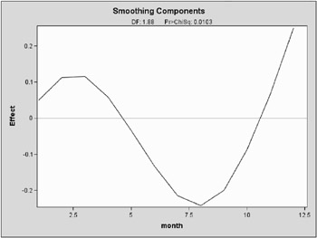
In Output 30.2.5, it is apparent that the pattern of repair rates follows the general pattern observed in Output 30.2.2. However, the plot of Output 30.2.5, is much cleaner as the month-to-month fluctuations are smoothed out to reveal the broader seasonal trend.
You can use the PLOTS(CLM) option to added a 95% confidence band to the plot of s ( Month j ), as in the following statements.
ods html; ods graphics on; proc gam data=equip plots(clm); model removals=spline(month) / dist=Poisson method=gcv; run; ods graphics off; ods html close;
The plot is displayed in Output 30.2.6.
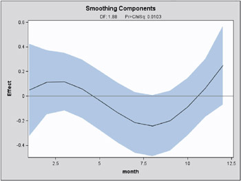
The small p -value in Output 30.2.1 of 0.0321 for the hypothesis of no seasonal trend indicates that the data exhibit significant seasonal structure. However, Output 30.2.6 is a graphical illustration of a degree of indistinctness in that structure. For instance, the horizontal reference line at zero is entirely within the 95% confidence band; that is, the estimated nonlinear part of the trend is relatively flat. Thus, despite evidence of seasonality based on the parametric model, it is difficult to narrow down its significant effects to a specific part of the year.
Example 30.3. Comparing PROC GAM with PROC LOESS
In an analysis of simulated data from a hypothetical chemistry experiment, additive nonparametric regression performed by PROC GAM is compared to the unrestricted multidimensional procedure of PROC LOESS.
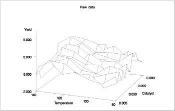
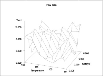
In each repetition of the experiment, a catalyst is added to a chemical solution, thereby inducing synthesis of a new material. The data are measurements of the temperature of the solution, the amount of catalyst added, and the yield of the chemical reaction. The following code reads and plots the raw data.
data ExperimentA; format Temperature f4.0 Catalyst f6.3 Yield f8.3; input Temperature Catalyst Yield @@; datalines; 80 0.005 6.039 80 0.010 4.719 80 0.015 6.301 80 0.020 4.558 80 0.025 5.917 80 0.030 4.365 80 0.035 6.540 80 0.040 5.063 80 0.045 4.668 80 0.050 7.641 80 0.055 6.736 80 0.060 7.255 80 0.065 5.515 80 0.070 5.260 80 0.075 4.813 80 0.080 4.465 90 0.005 4.540 90 0.010 3.553 90 0.015 5.611 90 0.020 4.586 90 0.025 6.503 90 0.030 4.671 90 0.035 4.919 90 0.040 6.536 90 0.045 4.799 90 0.050 6.002 90 0.055 6.988 90 0.060 6.206 90 0.065 5.193 90 0.070 5.783 90 0.075 6.482 90 0.080 5.222 100 0.005 5.042 100 0.010 5.551 100 0.015 4.804 100 0.020 5.313 100 0.025 4.957 100 0.030 6.177 100 0.035 5.433 100 0.040 6.139 100 0.045 6.217 100 0.050 6.498 100 0.055 7.037 100 0.060 5.589 100 0.065 5.593 100 0.070 7.438 100 0.075 4.794 100 0.080 3.692 110 0.005 6.005 110 0.010 5.493 110 0.015 5.107 110 0.020 5.511 110 0.025 5.692 110 0.030 5.969 110 0.035 6.244 110 0.040 7.364 110 0.045 6.412 110 0.050 6.928 110 0.055 6.814 110 0.060 8.071 110 0.065 6.038 110 0.070 6.295 110 0.075 4.308 110 0.080 7.020 120 0.005 5.409 120 0.010 7.009 120 0.015 6.160 120 0.020 7.408 120 0.025 7.123 120 0.030 7.009 120 0.035 7.708 120 0.040 5.278 120 0.045 8.111 120 0.050 8.547 120 0.055 8.279 120 0.060 8.736 120 0.065 6.988 120 0.070 6.283 120 0.075 7.367 120 0.080 6.579 130 0.005 7.629 130 0.010 7.171 130 0.015 5.997 130 0.020 6.587 130 0.025 7.335 130 0.030 7.209 130 0.035 8.259 130 0.040 6.530 130 0.045 8.400 130 0.050 7.218 130 0.055 9.167 130 0.060 9.082 130 0.065 7.680 130 0.070 7.139 130 0.075 7.275 130 0.080 7.544 140 0.005 4.860 140 0.010 5.932 140 0.015 3.685 140 0.020 5.581 140 0.025 4.935 140 0.030 5.197 140 0.035 5.559 140 0.040 4.836 140 0.045 5.795 140 0.050 5.524 140 0.055 7.736 140 0.060 5.628 140 0.065 6.644 140 0.070 3.785 140 0.075 4.853 140 0.080 6.006 ; title2 'Raw data'; proc g3d data=ExperimentA; plot Temperature*Catalyst=Yield / zmin=2 zmax=11; run;
The plot is displayed in Output 30.3.1.
The following code requests that both PROC LOESS and PROC GAM fit surfaces to the data.
ods output OutputStatistics=PredLOESS; proc loess data=ExperimentA; model Yield = Temperature Catalyst / scale=sd degree=2 select=gcv; run; ods output close; proc gam data=ExperimentA; model Yield = loess(Temperature) loess(Catalyst) / method=gcv; output out=PredGAM; run;
In both cases the smoothing parameter was chosen as the value that minimizes GCV. This is performed automatically by PROC LOESS and PROC GAM.
The following code generates plots of the predicted yields, which are displayed in Output 30.3.2.
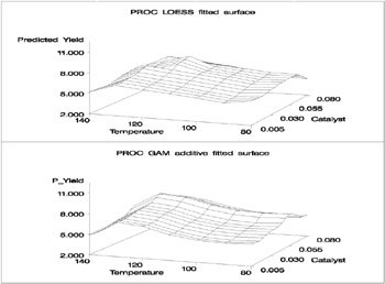
title2 'PROC LOESS fitted surface'; proc g3d data=PredLOESS; format pred f6.3; plot Temperature*Catalyst=pred / name='LOESSA' zmin=2 zmax=11; run; title2 'PROC GAM additive fitted surface'; proc g3d data=PredGAM; format P_Yield f6.3; plot Temperature*Catalyst=P_Yield / name='GAMA' zmin=2 zmax=11; run; goptions display; proc greplay nofs tc=sashelp.templt template=v2 ; igout=gseg; treplay 1:loessa 2:gama; run; quit;
Though both PROC LOESS and PROC GAM use the statistical technique loess, it is apparent from Output 30.3.2 that the manner in which it is applied is very different. By smoothing out the data in local neighborhoods, PROC LOESS essentially fits a surface to the data in pieces, one neighborhood at a time. The local regions are treated independently, so separate areas of the fitted surface are only weakly re-lated. PROC GAM imposes additive structure, requiring that cross sections of the fitted surface always have the same shape and thereby relating regions that have a common value of the same individual regressor variable. Under that restriction, the loess technique need not be applied to the entire multidimensional scatter plot, but only to one-dimensional cross sections of the data.
The advantage of using additive model fitting is that its statistical power is directed toward univariate smoothing, and so it is able to discern the finer details of any underlying structure in the data. Regression data may be very sparse when viewed in the context of multidimensional space, even when every individual set of regressor values densely covers its range. This is the familiar curse of dimensionality. Sparse data greatly restricts the effectiveness of nonparametric procedures, but additive model fitting, when appropriate, is one way to overcome this limitation.
To examine these properties, plots of cross sections of unrestricted (PROC LOESS) and additive (PROC GAM) fitted surfaces for the variable Catalyst are generated by the following code. The code for creating the cross section plots and overlaying them is somewhat complicated, so a macro %XPlot is employed to make it easy to create this plot for the results of each procedure.
axis1 minor=none order=(2 to 11 by 2) label=(angle=90 rotate=0 "Predicted Yield"); axis2 minor=none order=(0.005 to 0.080 by 0.02 5) label=("Catalyst"); symbol1 color=blue interpol=join value=none line=1 width=1; %macro XPLOT(proc=,name=); proc sort data=Pred&proc; by Catalyst Temperature; run; data PredX&proc; keep Pred80 Pred90 Pred100 Pred110 Pred120 Pred130 Pred140 Catalyst; array xPred{8:14} Pred80 Pred90 Pred100 Pred110 Pred120 Pred130 Pred140; retain Pred80 Pred90 Pred100 Pred110 Pred120 Pred130 Pred140; set Pred&proc; %if &proc=LOESS %then %do; xPred{Temperature/10} = pred; %end; %else %if &proc=GAM %then %do; xPred{Temperature/10} = P_Yield; %end; if abs(Temperature-140)<1 then output; run; proc gplot data=PredX&proc; plot Pred140*Catalyst=1 Pred130*Catalyst=1 Pred120*Catalyst=1 Pred110*Catalyst=1 Pred100*Catalyst=1 Pred90*Catalyst=1 Pred80*Catalyst=1 / overlay cframe=ligr name=&name vaxis=axis1 haxis=axis2; run; quit; %mend; title; title2 'PROC LOESS fitted surface, cross sections'; %XPLOT(proc=LOESS,name='XLOESSA'); title2 'PROC GAM additive fitted surface, cross sections'; %XPLOT(proc=GAM,name='XGAMA'); goptions display; proc greplay nofs tc=sashelp.templt template=v2 ; igout=gseg; treplay 1:xloessa 2:xgama; run; quit; The plots are displayed in Output 30.3.3.
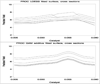
Notice that the graphs in the top panel (PROC LOESS) of Output 30.3.3 have varying shapes , while every graph in the bottom panel (PROC GAM) is the same curve shifted vertically. This illustrates precisely the kind of structural differences that distinguish additive models. A second important comparison to make in Output 30.3.2 and Output 30.3.3 is the level of detail in the fitted regression surfaces. Cross sections of the PROC LOESS surface are rather flat, but those of the additive surface have a clear shape. In particular, the ridge near Catalyst=0.055 is only vaguely evident in the PROC LOESS surface, but it is plainly revealed by the additive procedure.
For an example of a situation where unrestricted multidimensional fitting is preferred over additive regression, consider the following simulated data from a similar experiment. The following code creates another SAS data set and plot.
data ExperimentB; format Temperature f4.0 Catalyst f6.3 Yield f8.3; input Temperature Catalyst Yield @@; datalines; 80 0.005 9.115 80 0.010 9.275 80 0.015 9.160 80 0.020 7.065 80 0.025 6.054 80 0.030 4.899 80 0.035 4.504 80 0.040 4.238 80 0.045 3.232 80 0.050 3.135 80 0.055 5.100 80 0.060 4.802 80 0.065 8.218 80 0.070 7.679 80 0.075 9.669 80 0.080 9.071 90 0.005 7.085 90 0.010 6.814 90 0.015 4.009 90 0.020 4.199 90 0.025 3.377 90 0.030 2.141 90 0.035 3.500 90 0.040 5.967 90 0.045 5.268 90 0.050 6.238 90 0.055 7.847 90 0.060 7.992 90 0.065 7.904 90 0.070 10.184 90 0.075 7.914 90 0.080 6.842 100 0.005 4.497 100 0.010 2.565 100 0.015 2.637 100 0.020 2.436 100 0.025 2.525 100 0.030 4.474 100 0.035 6.238 100 0.040 7.029 100 0.045 8.183 100 0.050 8.939 100 0.055 9.283 100 0.060 8.246 100 0.065 6.927 100 0.070 7.062 100 0.075 5.615 100 0.080 4.687 110 0.005 3.706 110 0.010 3.154 110 0.015 3.726 110 0.020 4.634 110 0.025 5.970 110 0.030 8.219 110 0.035 8.590 110 0.040 9.097 110 0.045 7.887 110 0.050 8.480 110 0.055 6.818 110 0.060 7.666 110 0.065 4.375 110 0.070 3.994 110 0.075 3.630 110 0.080 2.685 120 0.005 4.697 120 0.010 4.268 120 0.015 6.507 120 0.020 7.747 120 0.025 9.412 120 0.030 8.761 120 0.035 8.997 120 0.040 7.538 120 0.045 7.003 120 0.050 6.010 120 0.055 3.886 120 0.060 4.897 120 0.065 2.562 120 0.070 2.714 120 0.075 3.141 120 0.080 5.081 130 0.005 8.729 130 0.010 7.460 130 0.015 9.549 130 0.020 10.049 130 0.025 8.131 130 0.030 7.553 130 0.035 6.191 130 0.040 6.272 130 0.045 4.649 130 0.050 3.884 130 0.055 2.522 130 0.060 4.366 130 0.065 3.272 130 0.070 4.906 130 0.075 6.538 130 0.080 7.380 140 0.005 8.991 140 0.010 8.029 140 0.015 8.417 140 0.020 8.049 140 0.025 4.608 140 0.030 5.025 140 0.035 2.795 140 0.040 3.123 140 0.045 3.407 140 0.050 4.183 140 0.055 3.750 140 0.060 6.316 140 0.065 5.799 140 0.070 7.992 140 0.075 7.835 140 0.080 8.985 ; run; title2 'Raw data'; proc g3d data=ExperimentB; plot Temperature*Catalyst=Yield / zmin=2 zmax=11; run;
A plot of the raw data is displayed in Output 30.3.4.
The SAS code for fitting the new data is essentially the same as that for the data set from the first experiment. Similar to Output 30.3.2, multivariate and additive fitted surfaces for these data are displayed in Output 30.3.5.

It is clear from Output 30.3.5 that the results of PROC LOESS and PROC GAM are completely different. While the plot in the top panel resembles the raw data plot in Output 30.3.4, the plot in the bottom panel is essentially featureless.
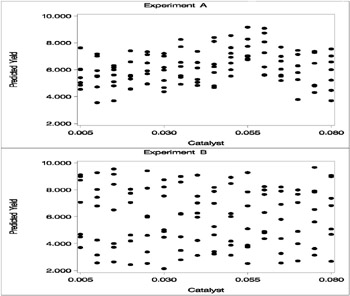
To understand what is happening, compare the scatter plots of Yield by Catalyst for the two data sets in this example. These are generated by the following code and displayed in Output 30.3.6.
| |
| |
axis1 minor=none order=(2 to 11 by 2) label=(angle=90 rotate=0 "Predicted Yield"); axis2 minor=none order=(0.005 to 0.080 by 0.025) label=("Catalyst"); symbol2 c=yellow v=dot i=none; title2 'Experiment A'; proc gplot data=ExperimentA; plot Yield*Catalyst=2 / cframe=ligr name='ExptA' vaxis=axis1 haxis=axis2; run; quit; title2 'Experiment B'; proc gplot data=ExperimentB; plot Yield*Catalyst=2 / cframe=ligr name='ExptB' vaxis=axis1 haxis=axis2; run; quit; proc greplay nofs tc=sashelp.templt template=v2; igout=gseg; treplay 1:expta 2:exptb; run; quit; The top panel of Output 30.3.6 hints at the same kind of structure exhibited in the fitted cross sections of Output 30.3.3. In PROC GAM, the additive model component corresponding to Catalyst is fit to a similar scatter plot, with the partial residuals computed in the backfitting algorithm, so it is able to capture the trend seen here. In contrast, when the second data set is viewed from the perspective of Output 30.3.6, the diagonal ridge apparent in Output 30.3.4 is washed out, and no clear structure shows up in the scatter plot. As a result, the additive model fit produced by PROC GAM is relatively featureless.