Statistical Analysis of Simulation Results

[Page 632 ( continued )]

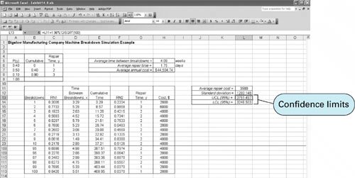
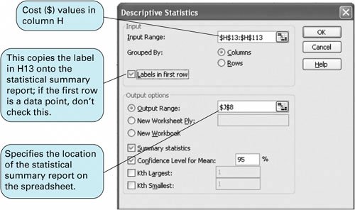
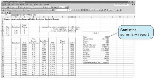
In general, the outcomes of a simulation model are statistical measures such as averages, as in the examples presented in this chapter. In our ComputerWorld example, we generated average revenue as a measure of the system we simulated; in the Burlingham Mills queuing example, we generated the average waiting time for batches to be dyed; and in the Bigelow Manufacturing Company machine breakdown example, the system was measured in terms of average repair costs. However, we also discussed the care that must be taken in accepting the accuracy of these statistical results because they were frequently based on relatively few observations (i.e., simulation replications). Thus, as part of the simulation process, these statistical results are typically subjected to additional statistical analysis to determine their degree of accuracy.

One of the most frequently used tools for the analysis of the statistical validity of simulations results is confidence limits. Confidence limits can be developed within Excel for the averages resulting from simulation models in several different ways. Recall that the statistical formulas for 95% confidence limits are

where is the mean and s is the sample standard deviation from a sample of size n from any population. Although we cannot be sure that the sample mean will exactly equal the population mean, we can be 95% confident that the true population mean will be between the upper confidence limit (UCL) and lower confidence limit (LCL) computed using these formulas.

Exhibit 14.9 shows the Excel spreadsheet for our machine breakdown example (from Exhibit 14.8), with the upper and lower confidence limits for average repair cost in cells L13 and L14. Cell L11 contains the average repair cost (for each incidence of a breakdown), computed by using the formula = AVERAGE(H14:H113 ). Cell L12 contains the sample standard deviation, computed by using the formula = STDEV(H14:H113 ). The upper confidence limit is computed in cell L13 by using the formula shown on the formula bar at the top of the spreadsheet, and the lower control limit is computed similarly. Thus, we can be 95% confident that the true average repair cost for the population is between $3,248.50 and $3,751.50.

---

[Page 633]

Exhibit 14.9.

Confidence limits plus several additional statistics can also be obtained by using the "Data Analysis" option from the "Tools" menu. (If this option is not available on your "Tools" menu, select the "Add-ins" option from the "Tools" menu and then select the "Analysis ToolPak" option.) Select the "Data Analysis" option from the "Tools" menu at the top of the spreadsheet, and then from the resulting menu select "Descriptive Statistics." This will result in a dialog box like the one shown in Exhibit 14.10. This box, completed as shown, results in the summary statistics for repair costs shown in cells J8:K23 in Exhibit 14.11. These summary statistics include the mean, standard deviation, and confidence limits we computed in Exhibit 14.9, plus several other statistics.

Exhibit 14.10.

---

[Page 634]

Exhibit 14.11.