Computer Simulation with Excel Spreadsheets | Introduction to Management Science (10th Edition)

[Page 617 ( continued )]

The simulation we performed manually for the ComputerWorld example was not too difficult. However, if we had performed the simulation for 1,000 weeks, it would have taken several hours. On the other hand, this simulation could be done on a computer in several seconds. Also, our simulation example was not very complex. As simulation models get progressively more complex, it becomes virtually impossible to perform them manually, thus making the computer a necessity.

Simulations are normally done on the computer .

Although we will not develop a simulation model in a computer language for this example, we will demonstrate how a computerized simulation model is developed by using Excel spreadsheets.

The first step in developing a simulation model is to generate a random number, r . Numerous subroutines that are available on practically every computer system generate random numbers. Most are quite easy to use and require the insertion of only a few statements in a program. These random numbers are generated by mathematical processes as opposed to a physical process, such as spinning a roulette wheel. For this reason, they are referred to as pseudorandom numbers . It should be apparent from the previous discussion that random numbers play a very important part in a probabilistic simulation. Some of the random numbers we used came from Table 14.3, a table of random numbers. However, random numbers do not come just from tables, and their generation is not as simple as one might initially think. If random numbers are not truly random, the validity of simulation results can be significantly affected.

[Page 618]

Random numbers generated by a mathematical process instead of a physical process are pseudorandom numbers .

The random numbers in Table 14.3 were generated by using a numerical technique . Thus, they are not true random numbers but pseudorandom numbers . True random numbers can be produced only by a physical process, such as spinning a roulette wheel over and over. However, a physical process, such as spinning a roulette wheel, cannot be conveniently employed in a computerized simulation model. Thus, there is a need for a numerical method that artificially creates random numbers.

Random numbers are typically generated on the computer by using a numerical technique .

To truly reflect the system being simulated, the artificially created random numbers must have the following characteristics:

The random numbers must be uniformly distributed. This means that each random number in the interval of random numbers (i.e., 0 to 1 or 0 to 100) has an equal chance of being selected. If this condition is not met, then the simulation results will be biased by the random numbers that have a more likely chance of being selected.
The numerical technique for generating random numbers should be efficient. This means that the random numbers should not degenerate into constant values or recycle too frequently.
The sequence of random numbers should not reflect any pattern. For example, the sequence of numbers 0, 1, 2, 3, 4, 5, 6, 7, 8, 9, 0, 1, 2, 3, 4, 5, 6, 7, 8, 9, 0, 1, 2, 3, 4, 5, 6, 7, 8, 9, 0, and so on, although uniform, is not random.

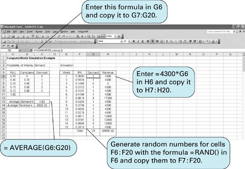
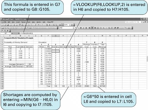
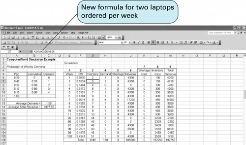
A table of random numbers must be uniform, efficiently generated, and absent of patterns .

Random numbers between 0 and 1 can be generated in Excel by entering the formula = RAND () in a cell . The random numbers generated by this formula include all the necessary characteristics for randomness and uniformity that we discussed earlier. Exhibit 14.1 is an Excel spreadsheet with 100 random numbers generated by entering the formula = RAND () in cell A3 and copying to the cells in the range A3:J12 . Recall that we can copy things in a range of cells in two ways. You can first cover cells A3:J12 with the cursor and then type the formula = RAND () into cell A3. Then you press the "Ctrl" and "Enter" keys simultaneously . Alternatively, you can type = RAND () in cell A3, copy this cell (using the right mouse button), then cover cells A3:J12 with the cursor, and (again with the right mouse button) paste this formula in these cells.

Exhibit 14.1.

If you attempt to replicate this spreadsheet, you will generate different random numbers from those shown in Exhibit 14.1. Every time you generate random numbers, they will be different. In fact, any time you recalculate anything on your spreadsheet, the random numbers will change. You can see this by pressing the F9 key and observing that all the random numbers change. However, sometimes it is useful in a simulation model to be able to use the same set (or stream) of random numbers over and over. You can freeze the random numbers you are using on your spreadsheet by first covering the cells with random numbers in them with the cursorfor example, cells A3:J12 in Exhibit 14.1. Next, you copy these cells (using the right mouse button); then you click on the "Edit" menu at the top of your spreadsheet and select "Paste Special" from this menu. Next, you select the "Values" option and click on "OK." This procedure pastes a copy of the numbers in these cells over the same cells with = RAND () formulas in them, thus freezing the numbers in place.

[Page 619]

Notice one more thing from Exhibit 14.1: The random numbers are all between 0 and 1, whereas the random numbers in Table 14.3 are whole numbers between 0 and 100. We used whole random numbers previously for illustrative purposes; however, computer programs such as Excel generally provide random numbers between 0 and 1.

Now we are ready to duplicate our example simulation model for the ComputerWorld store by using Excel. The spreadsheet in Exhibit 14.2 includes the simulation model originally developed in Table 14.4.

Exhibit 14.2.

Note that the probability distribution for the weekly demand for laptops has been entered in cells A6:C10 . Also notice that we have entered a new set of cumulative probability values in column B. We generated these cumulative probabilities by first entering 0 in cell B6, then entering the formula = A6+B6 in cell B7, and copying this formula to cells B8:B10 . This cumulative probability creates a range of random numbers for each demand value. For example, any random number less than 0.20 will result in a demand value of 0, and any random number greater than 0.20 but less than 0.60 will result in a demand value of 1, and so on. (Notice that there is no value of 1.00 in cell B11; the last demand value, 4, will be selected for any random number equal to or greater than .90.)

Random numbers are generated in cells F6:F20 by entering the formula = RAND () in cell F6 and copying it to the range of cells in F7:F20 .

[Page 620]

Now we need to be able to generate demand values for each of these random numbers in column F. We accomplish this by first covering the cumulative probabilities and the demand values in cells B6:C10 with the cursor. Then we give this range of cells the name "Lookup." This can be done by typing "Lookup" directly on the formula bar in place of B6 or by clicking on the "Insert" button at the top of the spreadsheet and selecting "Name" and "Define" and then entering the name "Lookup." This has the effect of creating a table called "Lookup" with the ranges of random numbers and associated demand values in it. Next, we enter the formula = VLOOKUP(F6,Lookup,2 ) in cell G6 and copy it to the cells in the range G7:G20 . This formula will compare the random numbers in column F with the cumulative probabilities in B6:B10 and generate the correct demand value from cells C6:C10 .

Once the demand values have been generated in column G, we can determine the weekly revenue values by entering the formula = 4300*G6 in H6 and copying it to cells H7:H20 .

Average weekly demand is computed in cell C13 by using the formula = AVERAGE(G6:G20) , and the average weekly revenue is computed by entering a similar formula in cell C14.

Notice that the average weekly demand value of 1.53 in Exhibit 14.2 is different from the simulation result (2.07) we obtained from Table 14.4. This is because we used a different stream of random numbers. As mentioned previously, to acquire an average closer to the true steady-state value, the simulation probably needs to include more repetitions than 15 weeks. As an example, Exhibit 14.3 simulates demand for 100 weeks. The window has been "frozen" at row 16 and scrolled up to show the first 10 weeks and the last 6 weeks on the screen in Exhibit 14.3.

Exhibit 14.3.

Decision Making with Simulation

In our previous example, the manager of ComputerWorld acquired some useful information about the weekly demand and revenue for laptops that would be helpful in making a decision about how many laptops would be needed each week to meet demand. However, this example did not lead directly to a decision. Next, we will expand our ComputerWorld store example so that a possible decision will result.

[Page 621]

From the simulation in Exhibit 14.3 the manager of the store knows that the average weekly demand for laptop PCs will be approximately 1.49; however, the manager cannot order 1.49 laptops each week. Because fractional laptops are not possible, either one or two must be ordered. Thus, the manager wants to repeat the earlier simulation with two possible order sizes, 1 and 2. The manager also wants to include some additional information in the model that will affect the decision.

If too few laptops are on hand to meet demand during the week, then not only will there be a loss of revenue, but there will also be a shortage cost of $500 per unit incurred because the customer will be unhappy . However, each laptop still in stock at the end of each week that has not been sold will incur an inventory or storage cost of $50. Thus, it costs the store money to have either too few or too many laptops on hand each week. Given this scenario, the manager wants to order either one or two laptops, depending on which order size will result in the greatest average weekly revenue.

Exhibit 14.4 shows the Excel spreadsheet for this revised example. The simulation is for 100 weeks. The columns labeled "1," "2," and "4" for "Week," "RN," and "Demand" were constructed similarly to the model in Exhibit 14.3. The array of cells B6:C10 was given the name "Lookup," and the formula = VLOOKUP(F6,Lookup,2 ) was entered in cell H6 and copied to cells H7:H105 .

Exhibit 14.4.

The simulation in Exhibit 14.4 is for an order size of one laptop each week. The "Inventory" column (3) keeps track of the amount of inventory available each weekthe one laptop that comes in on order plus any laptops carried over from the previous week. The cumulative inventory is computed each week by entering the formula = 1+MAX(G6H6,0 ) in cell G7 and copying it to cells G8:G105 . This formula adds the one laptop on order to either the number left over from the previous week ( G6-H6 ) or 0, if there were not enough laptops on hand to meet demand. It does not allow for negative inventory levels, called back orders . In other words, if a sale cannot be made due to a shortage, then it is gone. The inventory values in column 3 are eventually multiplied by the inventory cost of $50 per unit in column 8, using the formula = G6*50 .

[Page 622]

If there is a shortage, it is recorded in column 5, labeled "Shortage." The shortage is computed by entering the formula = MIN(G6-H6,0 ) in cell I6 and copying it to cells I7:I105 . Shortage costs are computed in column 7 by multiplying the shortage values in column 5 by $500 by entering the formula = I6*500 in cell K6 and copying it to cells K7:K105 .

Weekly revenues are computed in column 6 by entering the formula = 4300* MIN(H6,G6 ) in cell J6 and copying it to cells J7:J105 . In other words, the revenue is determined by either the inventory level in column 3 or the demand in column 4, whichever is smaller.

Total weekly revenue is computed in column 9 by subtracting shortage costs and inventory costs from revenue by entering the formula = J6-K6-L6 in cell M6 and copying it to cells M7:M105 .

The average weekly demand, 1.50, is shown in cell C13. The average weekly revenue, $3,875, is computed in cell C14.

Next, we must repeat this same simulation for an order size of two laptops each week. The spreadsheet for an order size of two is shown in Exhibit 14.5. Notice that the only actual difference is the use of a new formula to compute the weekly inventory level in column 3. This formula in cell G7, reflecting two laptops ordered each week, is shown on the formula bar at the top of the spreadsheet.

Exhibit 14.5.

This second simulation, in Exhibit 14.5, results in an average weekly demand of 1.50 laptops and an average weekly total revenue of $4,927.50. This is higher than the total weekly revenue of $3,875 achieved in the first simulation run in Exhibit 14.4, even though the store would incur significantly higher inventory costs. Thus, the correct decisionbased on weekly revenuewould be to order two laptops per week. However, there are probably additional aspects of this problem the manager would want to consider in the decision-making process, such as the increasingly high inventory levels as the simulation progresses. For example, there may not be enough storage space to accommodate this much inventory. Such questions as this and others can also be analyzed with simulation. In fact, one of the main attributes of simulation is its usefulness as a model for experimenting, called what-if? analysis .

[Page 623]

This example briefly demonstrates how simulation can be used to make a decision (i.e., to "optimize"). In this example we experimented with two order sizes and determined the one that resulted in the greater revenue. The same basic modeling principles can be used to solve larger problems with hundreds of possible order sizes and a probability distribution for demand with many more values plus variable lead times (i.e., the time it takes to receive an order), the ability to back order, and other complicating factors. These factors make the simulation model larger and more complex, but such models are frequently developed and used in business.