Decision Analysis with Additional Information | Introduction to Management Science (10th Edition)

[Page 538]

Earlier in this chapter we discussed the concept of the expected value of perfect information . We noted that if perfect information could be obtained regarding which state of nature would occur in the future, the decision maker could obviously make better decisions. Although perfect information about the future is rare, it is often possible to gain some amount of additional (imperfect) information that will improve decisions.

In this section we will present a process for using additional information in the decision-making process by applying Bayesian analysis . We will demonstrate this process using the real estate investment example employed throughout this chapter. Let's review this example briefly : A real estate investor is considering three alternative investments, which will occur under one of the two possible economic conditions (states of nature) shown in Table 12.11.

Table 12.11. Payoff table for the real estate investment example

	State of Nature
Decision (Purchase)	G OOD E CONOMIC C ONDITIONS .60	P OOR E CONOMIC C ONDITIONS .40
Apartment building	$ 50,000	$ 30,000
Office building	100,000	40,000
Warehouse	30,000	10,000

In Bayesian analysis additional information is used to alter the marginal probability of the occurrence of an event .

Recall that, using the expected value criterion, we found the best decision to be the purchase of the office building, with an expected value of $44,000. We also computed the expected value of perfect information to be $28,000. Therefore, the investor would be willing to pay up to $28,000 for information about the states of nature, depending on how close to perfect the information was.

Now suppose that the investor has decided to hire a professional economic analyst who will provide additional information about future economic conditions. The analyst is constantly researching the economy, and the results of this research are what the investor will be purchasing.

The economic analyst will provide the investor with a report predicting one of two outcomes . The report will be either positive, indicating that good economic conditions are most likely to prevail in the future, or negative, indicating that poor economic conditions will probably occur. Based on the analyst's past record in forecasting future economic conditions, the investor has determined conditional probabilities of the different report outcomes, given the occurrence of each state of nature in the future. We will use the following notations to express these conditional probabilities:

g = good economic conditions

p = poor economic conditions

P = positive economic report

N = negative economic report

A conditional probability is the probability that an event will occur, given that another event has already occurred .

[Page 539]

Management Science Application: Decision Analysis in the Electric Power Industry

Oglethorpe Power Corporation (OPC), a wholesale power generation and transmission cooperative, provides power to 34 consumer-owned distribution cooperatives in Georgia, representing 20% of the power in the state. Georgia Power Company meets the remaining power demand in Georgia. In general, Georgia has the ability to produce surplus power, whereas Florida, because of its rapidly growing population, must buy power from outside the state to meet its demand. In 1990, OPC learned that Florida Power Corporation wanted to add a transmission line to Georgia capable of transmitting an additional 1,000 milliwatts (mw). OPC had to decide whether to add this additional capacity at a cost of around $100 million, with annual savings of around $20 million or more. OPC used decision analysis and, specifically , decision trees to help make its ultimate decision. Decision analysis has become a very popular form of quantitative analysis in the electric power industry in the United States. OPC's decision tree analysis included a series of decisions combined with uncertainties. The initial decision alternatives in the tree were whether to build a new transmission line alone, build it in a joint venture with Georgia Power, or not build a new line at all. Subsequent decisions included whether to upgrade existing facilities to meet Florida's needs plus control of the new facilities. Uncertainties included construction costs, Florida's demand for power, competition from other power sellers to Florida, and the share of Florida power for which OPC would be able to contract. The full decision tree for this decision problem, including all combinations of decision nodes and probability nodes, includes almost 8,000 possible decision paths. The decision tree helped OPC understand its decision process better and enabled it to approach the problem so that it would understand its competitive situation with Florida Power Corporation to a greater extent before making a final decision.

Source: A. Borison, "Oglethorpe Power Corporation Decides about Investing in a Major Transmission System," Interfaces 25, no. 2 (MarchApril 1995): 2536.

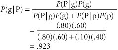
The conditional probability of each report outcome, given the occurrence of each state of nature, follows :

P (Pg) = .80

P (Ng) = .20

P (Pp) = .10

P (Np) = .90

For example, if the future economic conditions are, in fact, good (g), the probability that a positive report (P) will have been given by the analyst, P (Pg), is .80. The other three conditional probabilities can be interpreted similarly. Notice that these probabilities indicate that the analyst is a relatively accurate forecaster of future economic conditions.

The investor now has quite a bit of probabilistic information availablenot only the conditional probabilities of the report but also the prior probabilities that each state of nature will occur. These prior probabilities that good or poor economic conditions will occur in the future are

P (g) = .60

P (p) = .40

[Page 540]

Given the conditional probabilities, the prior probabilities can be revised to form posterior probabilities by means of Bayes's rule. If we know the conditional probability that a positive report was presented, given that good economic conditions prevail, P (Pg), the posterior probability of good economic conditions, given a positive report, P (gP), can be determined using Bayes's rule, as follows:

A posterior probability is the altered marginal probability of an event, based on additional information.

The prior probability that good economic conditions will occur in the future is .60. However, by obtaining the additional information of a positive report from the analyst, the investor can revise the prior probability of good conditions to a .923 probability that good economic conditions will occur. The remaining posterior (revised) probabilities are

P (gN) = .250

P (pP) = .077

P (pN) = .750

Decision Trees with Posterior Probabilities

The original decision tree analysis of the real estate investment example is shown in Figures 12.2 and 12.3. Using these decision trees, we determined that the appropriate decision was the purchase of an office building, with an expected value of $44,000. However, if the investor hires an economic analyst, the decision regarding which piece of real estate to invest in will not be made until after the analyst presents the report. This creates an additional stage in the decision-making process, which is shown in the decision tree in Figure 12.6. This decision tree differs in two respects from the decision trees in Figures 12.2 and 12.3. The first difference is that there are two new branches at the beginning of the decision tree that represent the two report outcomes. Notice, however, that given either report outcome, the decision alternatives, the possible states of nature, and the payoffs are the same as those in Figures 12.2 and 12.3.

Figure 12.6. Decision tree with posterior probabilities

(This item is displayed on page 541 in the print version)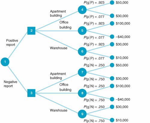

The second difference is that the probabilities of each state of nature are no longer the prior probabilities given in Figure 12.2; instead, they are the revised posterior probabilities computed in the previous section, using Bayes's rule. If the economic analyst issues a positive report, then the upper branch in Figure 12.6 (from node 1 to node 2) will be taken. If an apartment building is purchased (the branch from node 2 to node 4), the probability of good economic conditions is .923, whereas the probability of poor conditions is .077. These are the revised posterior probabilities of the economic conditions, given a positive report. However, before we can perform an expected value analysis using this decision tree, one more piece of probabilistic information must be determinedthe initial branch probabilities of positive and negative economic reports .

The probability of a positive report, P (P), and of a negative report, P (N), can be determined according to the following logic. The probability that two dependent events, A and B, will both occur is

P (AB) = P (AB) P (B)

If event A is a positive report and event B is good economic conditions, then according to the preceding formula,

P (Pg) = P (Pg) P (g)

[Page 541]

Management Science Application: Discount Fare Allocation at American Airlines

The management of its reservation system, referred to as yield management , is a significant factor in American Airlines's profitability. At American Airlines, yield management consists of three functions: overbooking, discount fare allocation, and traffic management. Overbooking is the practice of selling more reservations for a flight than there are available seats, to compensate for no-shows and cancellations . Discount allocation is the process of determining the number of discount fares to make available on a flight. Too few discount fares will leave a flight with empty seats, while too many will limit the number of flights to schedule to maximize revenues .

The process of determining the allocation of discount fares for a flight is essentially a decision analysis model with a decision tree. The initial decision is to accept or reject a discount fare request. If the initial decision is to reject the request, there is a probability, p , that the seat will eventually be sold at full fare and a probability, 1 p , that the seat will not be sold at all. The estimate of p is updated several times before flight departure , depending on the forecast for seat demand and the number of available seats remaining. If the expected value of the decision to rejectthat is, EV (reject discount fare) = ( p ) ($full fare)is greater than the discount fare, then the request is rejected.

Source: B. Smith, J. Leimkuhler, and R. Darrow, "Yield Management at American Airlines," Interfaces 22, no. 1 (JanuaryFebruary 1992): 831.

[Page 542]

We can also determine the probability of a positive report and poor economic conditions the same way:

P (Pp) = P (Pp) P (p)

Next, we consider the two probabilities P (Pg) and P (Pp), also called joint probabilities . These are, respectively, the probability of a positive report and good economic conditions and the probability of a positive report and poor economic conditions. These two sets of occurrences are mutually exclusive because both good and poor economic conditions cannot occur simultaneously in the immediate future. Conditions will be either good or poor, but not both. To determine the probability of a positive report, we add the mutually exclusive probabilities of a positive report with good economic conditions and a positive report with poor economic conditions, as follows:

P (P) = P (Pg) + P (Pp)

Events are mutually exclusive if only one can occur at a time .

Now, if we substitute into this formula the relationships for P (Pg) and P (Pp) determined earlier, we have

P (P) = P (Pg) P (g) + P (Pp) P (p)

You might notice that the right-hand side of this equation is the denominator of the Bayesian formula we used to compute P (gP) in the previous section. Using the conditional and prior probabilities that have already been established, we can determine that the probability of a positive report is

P (P) = P (Pg) P (g) + P (Pp) P (p) = (.80)(.60) + (.10)(.40) = .52

Similarly, the probability of a negative report is

P (N) = P (Ng) P (g) + P (Np) P (p) = (.20)(.60) + (.90)(.40) = .48

P (P) and P (N) are also referred to as marginal probabilities .

Now we have all the information needed to perform a decision tree analysis. The decision tree analysis for our example is shown in Figure 12.7. To see how the decision tree analysis is conducted , consider the result at node 4 first. The value $48,460 is the expected value of the purchase of an apartment building, given both states of nature. This expected value is computed as follows:

EV (apartment building) = $50,000(.923) + 30,000(.077) = $48,460

Figure 12.7. Decision tree analysis for real estate investment example

(This item is displayed on page 543 in the print version)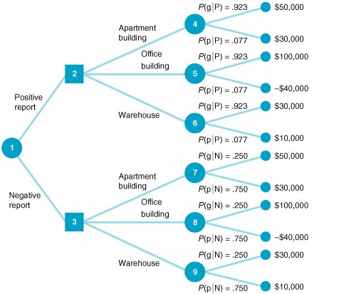

The expected values at nodes 5, 6, 7, 8, and 9 are computed similarly.

The investor will actually make the decision about the investment at nodes 2 and 3. It is assumed that the investor will make the best decision in each case. Thus, the decision at node 2 will be to purchase an office building, with an expected value of $89,220; the decision at node 3 will be to purchase an apartment building, with an expected value of $35,000. These two results at nodes 2 and 3 are referred to as decision strategies . They represent a plan of decisions to be made, given either a positive or a negative report from the economic analyst.

The final step in the decision tree analysis is to compute the expected value of the decision strategy, given that an economic analysis is performed. This expected value, shown as $63,194 at node 1 in Figure 12.7, is computed as follows:

This amount, $63,194, is the expected value of the investor's decision strategy, given that a report forecasting future economic condition is generated by the economic analyst.

[Page 543]

Computing Posterior Probabilities with Tables

One of the difficulties that can occur with decision analysis with additional information is that as the size of the problem increases (i.e., as we add more decision alternatives and states of nature), the application of Bayes's rule to compute the posterior probabilities becomes more complex. In such cases, the posterior probabilities can be computed by using tables. This tabular approach will be demonstrated with our real estate investment example. The table for computing posterior probabilities for a positive report and P (P) is initially set up as shown in Table 12.12.

Table 12.12. Computation of posterior probabilities

(1) State of Nature	(2) Prior Probability	(3) Conditional Probability	(4) Prior Probability x Conditional Probability: (2) x (3)	(5) Posterior Probability: (4) · S (4)
Good conditions	P (g) = .60	P (Pg) = .80	P (Pg) = .48
Poor conditions	P (p) = .40	P (Pp) = .10

The posterior probabilities for either state of nature (good or poor economic conditions), given a negative report, are computed similarly.

[Page 544]

No matter how large the decision analysis, the steps of this tabular approach can be followed the same way as in this relatively small problem. This approach is more systematic than the direct application of Bayes's "rule," making it easier to compute the posterior probabilities for larger problems.

Computing Posterior Probabilities with Excel

The posterior probabilities computed in Table 12.12 can also be computed by using Excel. Exhibit 12.16 shows Table 12.12 set up in an Excel spreadsheet format, as well as the table for computing P (N).

Exhibit 12.16.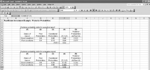

The Expected Value of Sample Information

Recall that we computed the expected value of our real estate investment example to be $44,000 when we did not have any additional information. After obtaining the additional information provided by the economic analyst, we computed an expected value of $63,194, using the decision tree in Figure 12.7. The difference between these two expected values is called the expected value of sample information (EVSI) , and it is computed as follows:

EVSI = EV _{with information} EV _{without information}

The expected value of sample information is the difference between the expected value with and without additional information .

For our example, the expected value of sample information is

EVSI = $63,194 44,000 = $19,194

This means that the real estate investor would be willing to pay the economic analyst up to $19,194 for an economic report that forecasted future economic conditions.

After we computed the expected value of the investment without additional information, we computed the expected value of perfect information , which equaled $28,000. However, the expected value of the sample information was only $19,194. This is a logical result because it is rare that absolutely perfect information can be determined. Because the additional information that is obtained is less than perfect, it will be worth less to the decision maker. We can determine how close to perfect our sample information is by computing the efficiency of sample information as follows:

efficiency = EVSI · EVPI = $19,194 / 28,000 = .69

The efficiency of sample information is the ratio of the expected value of sample information to the expected value of perfect information .

Thus, the analyst's economic report is viewed by the investor to be 69% as efficient as perfect information. In general, a high efficiency rating indicates that the information is very good, or close to being perfect information, and a low rating indicates that the additional information is not very good. For our example, the efficiency of .68 is relatively high; thus, it is doubtful that the investor would seek additional information from an alternative source. (However, this is usually dependent on how much money the decision maker has available to purchase information.) If the efficiency had been lower, however, the investor might seek additional information elsewhere.

[Page 545]

Management Science Application: Scheduling Refueling at the Indian Point 3 Nuclear Power Plant

The New York Power Authority (NYPA) owns and operates 12 power projects that provide roughly one-fourth of all the electricity used in New York State. Approximately 20% of NYPA's electrical power (supplying Westchester County and New York City) is generated by the Indian Point 3 (IP3) nuclear power plant, located on the Hudson River. IP3 withdraws 840,000 gallons of water per minute from the river for cooling steam and then returns it to the river. When water is withdrawn from the river , fish, especially small fish and eggs, do not always survive as they pass through the cooling system. The NYPA can reduce the negative effects by scheduling plant shutdowns to refuel IP3 when fish eggs and small fish are most abundant in the Hudson River. In the past, NYPA developed a refueling schedule according to a 10-year planning horizon, although unforeseen events often altered this schedule. There is uncertainty in the future about possible deregulation of the electric utility industry and its effect on the price of replacement power during refueling outages. The NYPA must consider these uncertainties in its attempt to provide low-cost power and minimize the environmental effects of refueling outages. The NYPA developed a decision analysis model to compare alternative strategies for refueling that balanced fish protection, the cost of buying fuel, and the uncertainties of deregulation .

The key decisions of the model were the times of year that refueling outages should occur, which affects the level of fish protection, and the amount of fuel that should be ordered for the nuclear reactor core that allows for operation for a target number of days, which affects the cost of the operation. The cost consideration comprises three objectives: minimizing the cost of replacement electricity when IP3 is shut down, minimizing the amount of unused fuel at the end of an operating cycle, and minimizing the time that IP3 would operate at less than full power before refueling. The objective of fish protection was to minimize the sum of the average percentage reduction in the mortality rate caused by water removal at IP3 for five types of fish over the 10-year planning horizon. The three major uncertainties in the model were the cost of refueling, how long it takes IP3 to refuel and how well it operates, and when New York State is likely to deregulate the electric utility industry. The decision analysis model considered five strategies based on different schedules that reflected different time windows when fish were most vulnerable. The model showed that no strategy simultaneously minimized refueling cost while minimizing fish mortality rates. The strategy that was selected restricted the starting date for refueling to the third week in May, when fish protection would meet accepted standards, at a cost savings of $10 million over the previous refueling schedule. The NYPA used the decision analysis model to develop its refueling schedule for the 10-year period from 1999 to 2008.

Source: D. J. Dunning, S. Lockfort, Q. E. Ross, P. C. Beccue, and J. S. Stonebraker, "New York Power Authority Uses Decision Analysis to Schedule Refueling of Its Indian Point 3 Nuclear Power Plant," Interfaces 31, no. 5 (SeptemberOctober 2001): 12135.